| (1) |
$Id: univar-analysis.tex,v 1.2 2003/08/11 22:27:05 greve Exp $
This document gives a terse description of how to perform linear univariate analysis of fMRI data (though the techniques generalize to other modalities). The name univariate is somewhat of a misnomer that has been adopted in fMRI. In this context, univariate refers to all the processing done on the time course from a single voxel, and multivariate refers to analysis done on multiple voxels (eg, Gaussian Random Fields). In this discussion, the observable is the raw data after any preprocessing (eg, slice-timing correction, motion correction, spatial smoothing). The techniques described are all linear2 in that the observable is modeled as a linear combination of regressors. The design matrix is the matrix whose columns are the regressors and contains information about the stimulus schedule, i.e., which stimulus was presented when. It may also have nuisance regressors (e.g., linear drift).
| (1) |
![]() is the
is the
![]() observable (1 = ``univariate'')
observable (1 = ``univariate'')
![]() is the
is the
![]() design matrix (stimulus convolution matrix)
design matrix (stimulus convolution matrix)
![]() is the
is the
![]() vector of regression coefficients (1 = ``univariate'')
vector of regression coefficients (1 = ``univariate'')
![]() is the noise variance
is the noise variance
![]() is
is
![]() noise covariance matrix; identity for
white noise.
noise covariance matrix; identity for
white noise.
![]() is the number of time points
is the number of time points
![]() is the number of regression coefficients
is the number of regression coefficients
The forward model represents a set of ![]() linear equations with
linear equations with
![]() unknowns (the
unknowns (the ![]() s).
s).
Assume white noise (
![]() ).
).
| (2) |
Signal Estimate:
| (3) |
Residual Error:
| (4) |
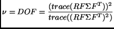
Degrees of Freedom:
| (5) |
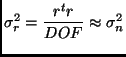
Residual Error Variance:
 |
(6) |
Covariance of
![]() under Null Hypothesis (
under Null Hypothesis (![]() ):
):
| (7) |
| (8) |
Contrast Effect Size:
| (9) |
t-Test (![]() ):
):
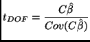 |
(10) |
F-Test:
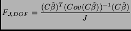 |
(11) |
| (12) |
| (13) |
Note: if a white noise model is assumed but the noise is not really white, then the statistics are said to be ``invalid'', meaning that the false positive rate (FPR) is not ideal. In fMRI, the FPR usually becomes ``liberal'' (ie, there are too many false positives).
Non-white noise and temporal filtering.
Forward Model with temporal filtering of the residuals:
| (14) |
New solution:
| (15) |
| (16) |
Residual Error forming Matrix:
| (17) |
Degrees of Freedom (Statistics):
Degrees of Freedom (Variance):
| (19) |
Residual Error Variance:
 |
(20) |
Covariance of
![]() under Null Hypothesis (
under Null Hypothesis (![]() ):
):
| (21) |
Make
![]() , make the smoothing induced by the
temporal filter much more than the inherent smoothness of the noise,
in which case:
, make the smoothing induced by the
temporal filter much more than the inherent smoothness of the noise,
in which case:
| (22) |
Setting
![]() is referred to as whitening
the residuals. Under this condition,
is referred to as whitening
the residuals. Under this condition,
![]() . This
results in a fully efficient estimator (ie,
. This
results in a fully efficient estimator (ie,
![]() ). Note that there are an infinite number of
). Note that there are an infinite number of ![]() 's that meet
the above condition. Typically
's that meet
the above condition. Typically ![]() is obtained from the Cholesky or
singular value decompositions.
is obtained from the Cholesky or
singular value decompositions.
In order to whiten, we need an estimate of ![]() . To do this, we
exploit the fact that the covariance matrix of a time-invariant
Gaussian process is a Toeplitz matrix of the autocorrelation
function, or ACF. This reduces estimating
. To do this, we
exploit the fact that the covariance matrix of a time-invariant
Gaussian process is a Toeplitz matrix of the autocorrelation
function, or ACF. This reduces estimating ![]() to estimating the
ACF of the noise. This is done by estimating the ACF of the
residuals. The ACF itself is often parameterized (eg, AR(1)). The ACF
is often very noisy, so it's usually a good idea to apply some spatial
regularization. Also, the residual ACF will be biased with respect to
the true ACF, though there are ways to compensate for this (Worsley,
et al, 2002).
to estimating the
ACF of the noise. This is done by estimating the ACF of the
residuals. The ACF itself is often parameterized (eg, AR(1)). The ACF
is often very noisy, so it's usually a good idea to apply some spatial
regularization. Also, the residual ACF will be biased with respect to
the true ACF, though there are ways to compensate for this (Worsley,
et al, 2002).
Goal: choose an event schedule (ie, an ![]() ) that will minimize the
expected sum-square error (SSE) of the estimates (
) that will minimize the
expected sum-square error (SSE) of the estimates (![]() ).
).
The error in ![]() is given by:
is given by:
| (23) |
The expected SSE is then
| (24) |
 |
(25) |
Algorithm: randomly select a stimulus schedule, compute ![]() , compute
the efficiency, do this a million times, keep the schedules that give
the largest efficiencies.
, compute
the efficiency, do this a million times, keep the schedules that give
the largest efficiencies.
The forward equation is
| (26) |
The event-related model (ERM) is best understood by first considering
a Finite-Impulse Response (FIR) model. The FIR makes no assumptions
about the shape of the hemodynamic response. In this model, a time window is hypothesized to exist around and event. The response
to the event is zero outside the window but can be anything in the
window (discretized to some sampling time). In the ![]() for the FIR,
the number of rows equals
for the FIR,
the number of rows equals ![]() (this is always the case) and the
number of columns equals the number of samples in the window
(
(this is always the case) and the
number of columns equals the number of samples in the window
(![]() ). This causes
). This causes ![]()
![]() to be interpreted as the value
of the response at the
to be interpreted as the value
of the response at the ![]() sample in the window. Example: for a
short event, the response may last for 20 sec, so one could start the
time window at
sample in the window. Example: for a
short event, the response may last for 20 sec, so one could start the
time window at ![]() (ie, stimulus onset) and end it at
(ie, stimulus onset) and end it at ![]() sampling at the TR (eg, TR=2). In this case,
sampling at the TR (eg, TR=2). In this case, ![]() . Note that if
the duration of the event is non-trivial, just extend the time window
to be long enough to capture the entire response. A blocked design is
just an event-related design with long events.
. Note that if
the duration of the event is non-trivial, just extend the time window
to be long enough to capture the entire response. A blocked design is
just an event-related design with long events.
The FIR ![]() is built in the following way. The components are either 0
or 1. The fist column is built by putting a 1 everywhere a stimulus
appears and a 0 everywhere else. The next column is the same as the
first but shifted down by one, filling the first row with a 0. Each
additional column constructed in the same way.
is built in the following way. The components are either 0
or 1. The fist column is built by putting a 1 everywhere a stimulus
appears and a 0 everywhere else. The next column is the same as the
first but shifted down by one, filling the first row with a 0. Each
additional column constructed in the same way.
Often one wants to make assumptions about the shape of the hemodynamic
response. Such assumptions can greatly increase the statistical power,
though there are some risks. In general, the ![]() matrix can be
computed as:
matrix can be
computed as:
| (27) |
Assuming a shape will usually increase the statistical power, sometimes dramatically so. To see why, consider assuming the shape using a simple gamma function. This model only has one free parameter: the amplitude. The equivalent FIR model may have 10 free parameters. Thus, for the gamma model, each event gives us an opportunity to observe that one parameter 10 times (approximately) whereas in the FIR, each parameter is only observed once. One roughly expects the variance of an estimated parameter to be reduced by a factor equal to the number of observations, so, all other things being equal, one expects the gamma parameter to have one tenth the variance of the FIR parameters. Note: this is why there is a penalty in the FIR model for extending the time window.
There are three main risks to assuming a shape to the hemodynamic
response; all have to due with mis-characterizing the shape. First, if
the true response is in the null space of ![]() , then
, then ![]() will be
zero, even in the case where there is no noise. In this case, all
statistical tests will report that there is no effect even though the
effect can be huge. The closer to the null space of
will be
zero, even in the case where there is no noise. In this case, all
statistical tests will report that there is no effect even though the
effect can be huge. The closer to the null space of ![]() the true
response is, the lower the final significance will be. Second,
mis-specifying the shape will cause the residual error to be larger;
but this is usually a small effect. The third risk is more difficult
to explain. If the assumed shape is wrong, then it cannot explain
all the signal associated with an event type. If the event schedules
are not thoroughly randomized, then the regressors from a second event
type can soak up some of the signal left by the first. This can make
the effect of the second event type appear to be larger than it
is. This can cause a false positive when compared to baseline or a
false negative when compared to the first stimulus. It is not known
how large this effect is.
the true
response is, the lower the final significance will be. Second,
mis-specifying the shape will cause the residual error to be larger;
but this is usually a small effect. The third risk is more difficult
to explain. If the assumed shape is wrong, then it cannot explain
all the signal associated with an event type. If the event schedules
are not thoroughly randomized, then the regressors from a second event
type can soak up some of the signal left by the first. This can make
the effect of the second event type appear to be larger than it
is. This can cause a false positive when compared to baseline or a
false negative when compared to the first stimulus. It is not known
how large this effect is.
If there are multiple event types, then build the
![]() matrix for each one and horizontally concatenate them together.
matrix for each one and horizontally concatenate them together.
A nuisance variable is generally considered to be any systematic
effect that is not part of the experimental paradigm. For example,
fMRI time courses always have a mean offset. Others include motion
artifacts and drift due to scanner heating. These effects can be
modeled by adding regressors to the design matrix. Ideally, the
nuisance regressors span the noise, thereby reducing the residual
variance and improving the statistical power. However, it is possible
(and likely) that the nuisance regressor will not be orthogonal to the
task-related components. When this happens, the task effect size may
drop significantly when the nuisance regressor is added. It is not
possible to say which task effect size is ``correct''.
The BOLD signal always has a mean offset that must be taken into
account when estimating the task-related effects. There can also be
slow increases/decreases due to amplifiers heating up, etc.
These effects can be accounted for in several ways. Here, we show how
to include polynomial regressors. The ![]() matrix will have
matrix will have ![]() rows
(always) and a number of columns equal to the
rows
(always) and a number of columns equal to the ![]() of the
polynomial, where
of the
polynomial, where ![]() is a constant (models the mean
offset). The first column will be all ones, the next will be linear
from 1 to
is a constant (models the mean
offset). The first column will be all ones, the next will be linear
from 1 to ![]() , the next will be quadratic, etc. Note that this will
be different than simply subtracting the mean from the raw time course
unless you also subtract the mean from the (non-polynomial) design
matrix. Once you have the
, the next will be quadratic, etc. Note that this will
be different than simply subtracting the mean from the raw time course
unless you also subtract the mean from the (non-polynomial) design
matrix. Once you have the ![]() for the polynomial regressors,
horizontally concatenate it with the design matrices from other
explanatory components.
for the polynomial regressors,
horizontally concatenate it with the design matrices from other
explanatory components.
When a functional volume is motion corrected, the program performing
the correction will output the six ``motion correction parameters''
for each volume in the series. These parameters are the translation
(3) and rotation at each time point. Together, they make an
![]() matrix. This matrix can be included as nuisance variables
(though it is best to do data reduction by taking the three largest
singular vectors). Given that the volume has been motion corrected,
why would you want to include motion correction regressors? The motion
correction algorithm cannot remove all the effects of motion. For
example, it cannot remove the spin history effect, which is when
tissue not in the original slice plane gets moved into the slice
plane. This tissue was not excited by the RF pulse and so will have no
signal. Note: using motion correction regressors can be tricky because
it is often the canse that the subject moves in time to the stimulus,
which causes the motion correction regressors to span the space of the
task-related signal. This can cause a drop in the task-related effect
size. On the other hand, if there is stimulus-locked motion, one does
not know whether an effect is due to motion or to stimulus. This is
much more likely to happen during a blocked design.
matrix. This matrix can be included as nuisance variables
(though it is best to do data reduction by taking the three largest
singular vectors). Given that the volume has been motion corrected,
why would you want to include motion correction regressors? The motion
correction algorithm cannot remove all the effects of motion. For
example, it cannot remove the spin history effect, which is when
tissue not in the original slice plane gets moved into the slice
plane. This tissue was not excited by the RF pulse and so will have no
signal. Note: using motion correction regressors can be tricky because
it is often the canse that the subject moves in time to the stimulus,
which causes the motion correction regressors to span the space of the
task-related signal. This can cause a drop in the task-related effect
size. On the other hand, if there is stimulus-locked motion, one does
not know whether an effect is due to motion or to stimulus. This is
much more likely to happen during a blocked design.
References:
Worsley, et al. A general statistical analysis for fMRI
Data. NeuroImage 15, 1-15 (2002).
This document was generated using the LaTeX2HTML translator Version 99.2beta8 (1.46)
Copyright © 1993, 1994, 1995, 1996,
Nikos Drakos,
Computer Based Learning Unit, University of Leeds.
Copyright © 1997, 1998, 1999,
Ross Moore,
Mathematics Department, Macquarie University, Sydney.
The command line arguments were:
latex2html -split 0 -nonavigation -dir univar-analysis univar-analysis.tex
The translation was initiated by Doug Greve on 2003-08-11