The purpose of this tutorial is to give you experience with the integration of Diffusion Tensor Imaging (DTI) with FreeSurfer. The data were collected at MGH as part of the MIND.
If you are looking for the Tracula tutorial, you can find it here.
DTI Basics
It is assumed that you already have some basic knowledge of DTI and its analysis. This paragraph is supplied as a summary for completeness. DTI attempts to measure the diffusion of water molecules in the tissue. Within the brain, white matter tracts tend to act like little straws that constrain the direction of diffusion. DTI analysis measures the orientation and "strength" of this orientation. For example, the CSF will have no strong orientation information. The strength of preferred orientation is often measured by fractional anisotropy (FA) and diffusivity is often measured by the Apparent Diffusion Coefficient (ADC).
Tutorial Data Set
This data was acquired at MGH as part of a MIND Consortium study. The raw data are in DICOM format (*.dcm) in the subject's 'orig' folder. Seventy images were acquired, 10 low-b and 60 diffusion weighted. The bvalues and gradient directions are stored in the DICOM header and are written to bvals.dat and bvects.dat, respectively, during the below analysis. The diffusion data are located in the $TUTORIAL_DATA/diffusion_tutorial directory and the corresponding FreeSurfer anatomical analysis (recon) is located in the $TUTORIAL_DATA/diffusion_recons directory. So when you start your data processing you should set the 'SUBJECTS_DIR' and 'TUTORIAL_DIR' path variables:
setenv SUBJECTS_DIR $TUTORIAL_DATA/diffusion_recon

setenv TUTORIAL_DIR $TUTORIAL_DATA/diffusion_tutorial
The examples are going to be demonstrated with respect to one particular subject. So in order to run the various commands successfully, you will need to define that as well. (If you want to run the tutorial steps on a different DTI tutorial subject, you can simply reset this variable.)
set subj = Diff001
This tutorial uses Freeview to view the output on several processing steps. Click here for background information on Freeview.
DTI Data Analysis Processing Stream
Pre-processing
The following steps are necessary to prepare the diffusion data for various types of analyses. On each step there is a description of the command and how it relates to the overall processing stream, the actual command you would use, and how to visualize the output. Similar pre-processing steps can be accomplished by using Tracula, although output will be generated using different file names and file types. You may find that you prefer one method over the other depending on the types of analyses and degree of involvement you want to have.
DT_Recon
To begin with you will need to reconstruct the diffusion tensor data from the DICOM files acquired by the MR scanner. Additionally, it is recommended to correct for Eddy currents and any motion artifacts, which could distort the DTI data. This pre-processing step uses the dt_recon command to accomplish this. It generates multiple NIFTI volumes that will be used in later steps. By default, the dt_recon command assumes that the FreeSurfer anatomical analysis (recon) has already been completed. If your diffusion DICOM files were acquired using a non-Siemens scanner, you will have to specify the scan specific bvalues and bvector with the '--b' flag. If your DICOM files were acquired using a Siemens scanner, then this information can be extracted from the DICOM headers and the bvalues and bvector files are saved in the bvals.dat and bvecs.dat files. The DICOM files in this tutorial data set were acquired using a Siemens scanner.
dt_recon --i $TUTORIAL_DIR/$subj/orig/*-1.dcm --s $subj --o $TUTORIAL_DIR/$subj/dtrecon
The location of the DICOM files for our subject is indicated by the '--i' flag. In the case of this tutorial, they are located in a sub-folder named 'orig' within each subject's main folder. In order to automatically establish a correspondence between the structural and diffusion scans of the same subject, we pass the subject ID information using the '--s' flag. That will allow the program to find the relevant files in '$SUBJECTS_DIR/$subj' of the structural recon. (If you do not have access to the structural recons at the time of the diffusion analysis, you can omit '--s' and use the '--no-reg' flag.) The desired location of the output is indicated with the '--o' flag. In this example, we are going to name the output folder 'dtrecon', which will be automatically created by the program.
This command has already been run for all of the subjects in the study. At a later time you may want to try running the command on a single subject from this tutorial, which will overwrite the output files, but should not affect the tutorial dataset.
To see a script which could be used to run the dt_recon on multiple subjects take a look at the 'DiffPreproc.csh' script on this page.
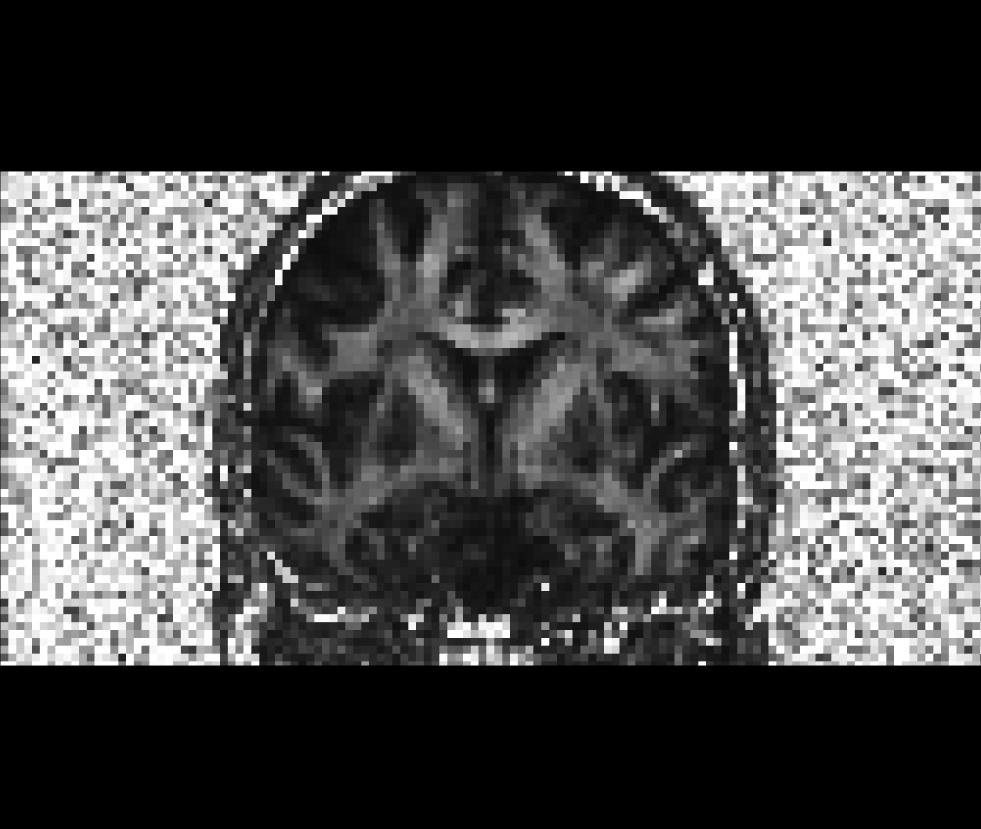
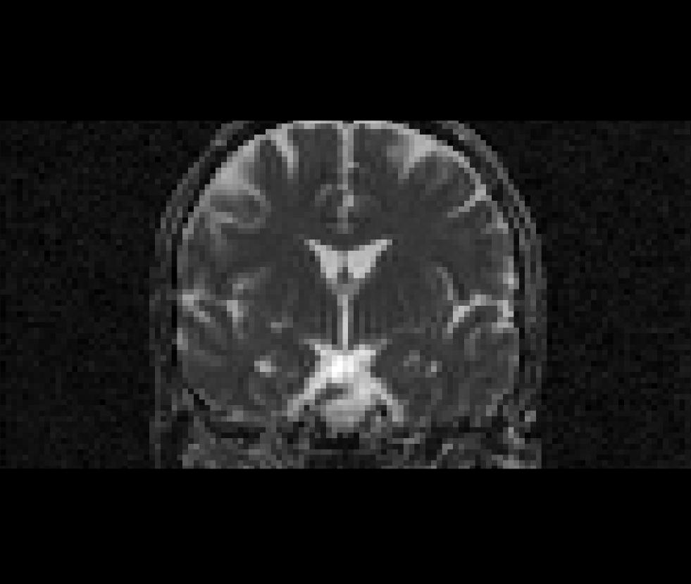
After running the 'dt_recon' command, you may want look at some of the outputs in Freeview. Run the following command to view the fractional anisotropy volume (fa.nii) and the apparent diffusion coefficient volume (adc.nii). The '$TUTORIAL_DIR' and '$subj' parameters need to be defined in advance. If you haven't done this already, please see the "Tutorial Data Set" section near the top of the page.
freeview -v $TUTORIAL_DIR/$subj/dtrecon/fa.nii \
            $TUTORIAL_DIR/$subj/dtrecon/adc.nii
Coronal view of the fractional anisotropy volume (fa.nii):
Coronal view of the apparent diffusion coefficient volume (adc.nii):
All other volumetric data sets generated by dt_recon (*.nii) could be viewed in a similar way. To see an explanation for the various volumes, see page
Resampling Structural Data in the Diffusion Space
In order to be able to refer to specific sub-cortical regions or areas of white matter in the diffusion data (and in the group analysis), we resample some of the segmentation volumes from the structural recon folder to the diffusion space. The registration between the diffusion and structural space has already been computed as part of the previous pre-processing step (unless you ran 'dt_recon' with the --no-reg flag). The 'registration.dat' file describes a rigid-body transformation from the diffusion to the structural space. As we would like to resample the structural volume into the structural space, we will need to apply the inverse of this transformation to our input volumes. We use the 'mri_vol2vol' command for this task. In the example below, we resample the white-matter parcellation volume (wmparc.mgz) into the diffusion space. Additionally, you may also want to repeat that process for the cortically-labelled volume segmentation (aparc+aseg.mgz).
mri_vol2vol --mov $TUTORIAL_DIR/$subj/dtrecon/lowb.nii --targ $SUBJECTS_DIR/$subj/mri/wmparc.mgz \
            --inv --interp nearest --o $SUBJECTS_DIR/$subj/mri/wmparc2diff.mgz \
            --reg $TURORIAL_DIR/$subj/dtrecon/register.dat --no-save-reg
Remember that in the above, it is the inverse transformation that we apply, so the role of the 'moving' and 'target' volumes are also going to be inverse. The input flags should be used to reflect the original direction of the transformation, and it is the '--inv' flag that will reverse their roles. When computing the 'register.dat' transformation, it was the 'lowb.nii' volume that was moved into the structural space, so we indicate this volume by the '--mov' flag. (Note, any diffusion related volume from the dt_recon file could be used here.) The target of the original registration was in the structural space and that is indicated by the '--targ' flag. As it is the wmparc.mgz volume that we wish to resample in the diffusion space, in the above, we identify the target volume to be that. The '--interp' flag indicates the type of interpolation that we want to use for the resampling. In the case of segmentation volumes, that option should always be set to nearest, indicating nearest neighbor interpolation. The '--o' flag indicates the desired output filename location, which in our example is 'wmparc2diff.mgz'. The rigid-body transformation matrix is stored in the register.dat file and it is indicated by the '--reg' flag. You can use the same 'register.dat' file to move other structural volumes of this subject into the same diffusion space. The '--no-save-reg' flag tells 'mri_vol2vol' not to write out another registration matrix file.
This command has been run for all of the subjects in the study for you already. At a later time you may want to try running the command on a single subject from this tutorial, which will overwrite the output files, but should not affect the tutorial dataset.
To see a script which could be used to run the mri_vol2vol command on multiple subjects using both the wmparc.mgz and aparc+aseg.mgz, take a look at the 'AlignAnat2Diff.csh' script on this page.
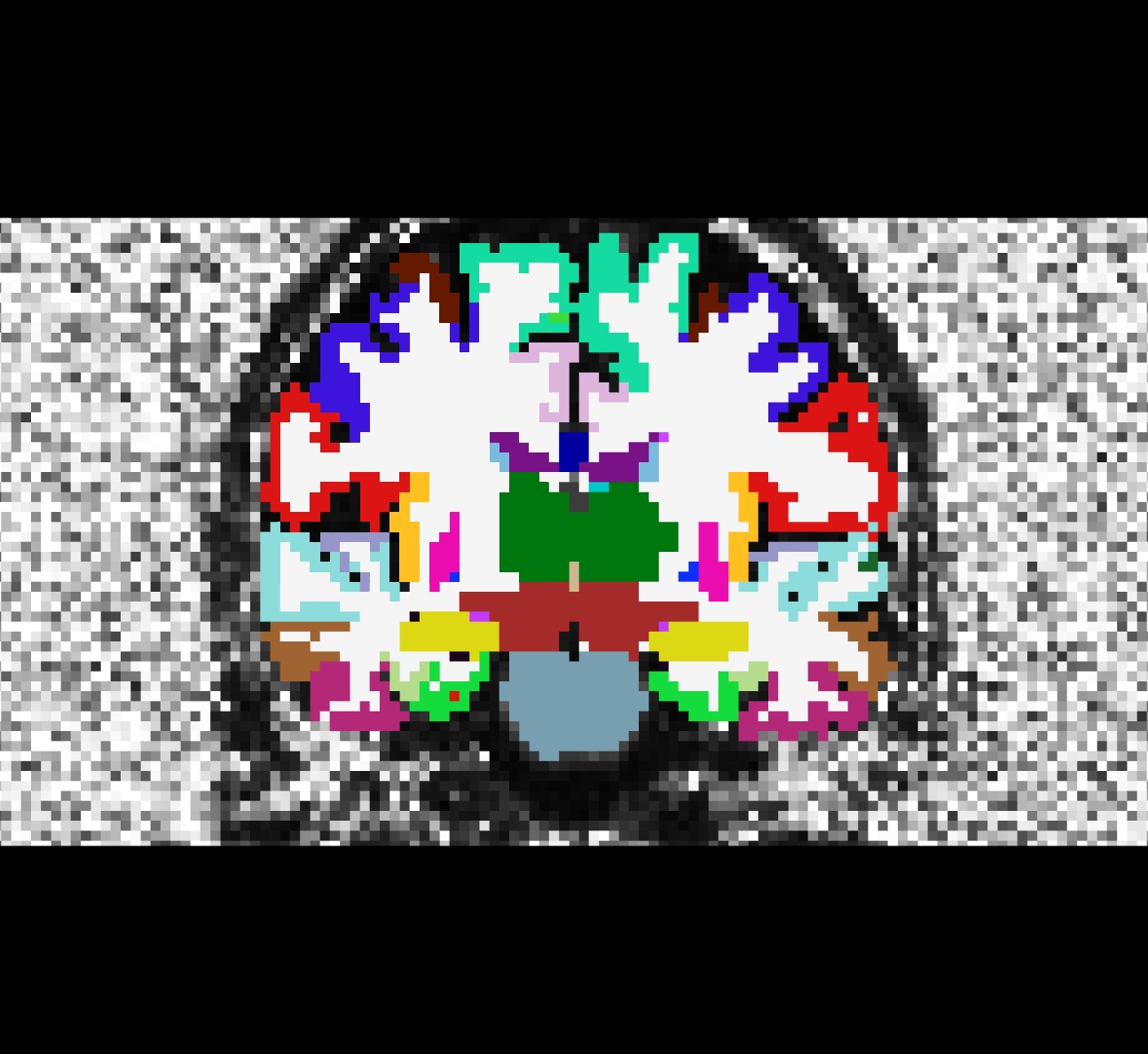
After running this command you may want look at the output in Freeview. Run the following command to view the aparc+aseg2diff.mgz overlayed on the fa.nii volume using a colormap lookup table (lut). The '$TUTORIAL_DIR', '$subj', and '$SUBJECTS_DIR' parameters need to be defined in advance. If you haven't done this already, please see the "Tutorial Data Set" section near the top of the page.
freeview -v $TUTORIAL_DIR/$subj/dtrecon/fa.nii \
            $SUBJECTS_DIR/$subj/mri/aparc+aseg2diff.mgz:colormap=lut
Coronal view of the cortically-labelled volume segmentation (aparc+aseg2diff.mgz) overlayed on the fractional anistropy volume (fa.nii):
Masking
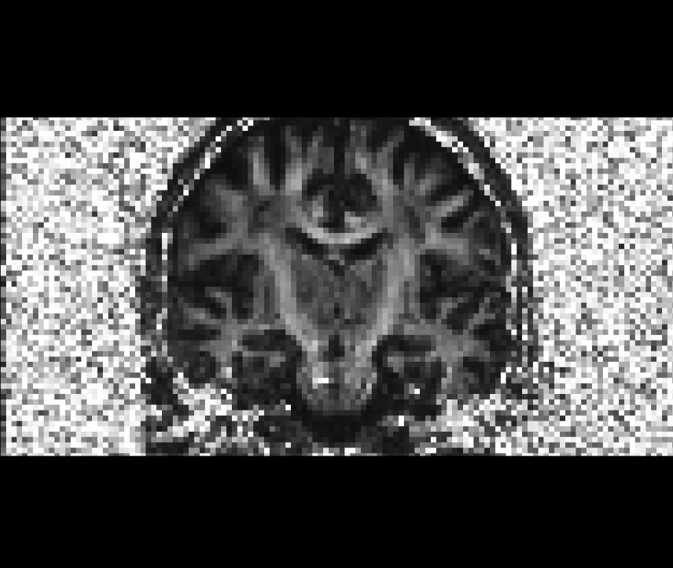
You may have noticed that there is some unwanted "noise" or "speckles" in the diffusion images when we view them in Freeview. This can be removed by masking out the space surrounding the brain. We will use one of the segmentation volumes from the recon directory that is already resampled in the diffusion space (wmparc2diff.mgz) as the mask. This way all non-brain areas will be assigned to the background. This step uses the 'mri_mask' command to remove the unwanted "noise". The difference should be clear by examining a volume before and after masking (see the Freeview commands below). The command below applies a mask to the fractional anisotropy volume (fa.nii), but you may run 'mri_mask' on any other diffusion volume (i.e., adc.nii, ivc.nii)
mri_mask $TUTORIAL_DIR/$subj/dtrecon/fa.nii $SUBJECTS_DIR/$subj/mri/wmparc2diff.mgz \
         $TUTORIAL_DIR/$subj/dtrecon/fa-masked.mgz
This command does not require flags to be passed, you just need to verify the order of the input arguments you are passing to it. The first argument should be the volume you wish to mask. The second argument is the volume to be used as a mask. And the third argument should be the name of the output file you would like to be created. In this example, we append '-masked' to the original unmasked volume file name so we can tell them apart.
This command has been run for all of the subjects in the study for you already. At a later time you may want to try running the command on a single subject from this tutorial, which will overwrite the output files, but should not affect the tutorial dataset.
To see a script which could be used to run the mri_mask command on multiple subjects take a look at the 'DiffMasking.csh' script on this page.
After running this command you may want look at the output in Freeview. Run the following command to compare the fractional anisotropy volume (fa.nii) before and after masking using the white matter parcelation volume (wmparc2diff.mgz), which we resampled earlier into diffusion space. The '$TUTORIAL_DIR' and '$subj' parameters need to be defined in advance. If you haven't done this already, please see the "Tutorial Data Set" section near the top of the page.
freeview –v $TUTORIAL_DIR/$subj/dtrecon/fa.nii \
            $TUTORIAL_DIR/$subj/dtrecon/fa-masked.mgz
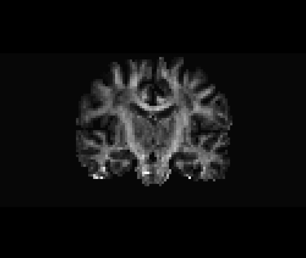
Coronal view of the unmasked fractional anisotropy volume (fa.nii):
Coronal view of the masked fractional anisotropy volume (fa-masked.mgz):
Spatial Normalization
At this point we could run analyses with a subject's own DTI and structural data, but we could not do a voxel-based group analysis with multiple subjects, because the data sets are not yet aligned in a common coordinate space. In other words, a certain coordinate location in one subject's volume does not necessarily correspond to the same anatomical location in any of our other subjects. This step normalizes (resamples) the diffusion data of one subject to a specified common coordinate space. In this example, the data will be resampled in CVS space, but alternatively you could normalize your data in any other (for example, MNI or Talairach). As a result of running mri_cvs_register on the structural acquisitions, an m3z morph file ('combined_toavg35rerun_elreg_afteraseg-norm.m3z') describes the transformation for each subject that is necessary to move from an individual's native space to that of the common CVS space.
mri_vol2vol --targ $FREESURFER_HOME/subjects/cvs_avg35/mri/norm.mgz \
            --m3z $SUBJECTS_DIR/$subj/cvs/combined_toavg35rerun_elreg_afteraseg-norm.m3z \
            --noDefM3zPath --reg $TUTORIAL_DIR/$subj/dtrecon/register.dat \
            --mov $TUTORIAL_DIR/$subj/dtrecon/fa-masked.nii --o $TUTORIAL_DIR/$subj/dtrecon/fa-masked.ANAT+CVS-to-avg35.mgz \
            --interp trilin --no-save-reg
The target CVS space where we want to resample our input volume (fa-masked.mgz) is indicated with the '--targ' flag. The '--m3z' flag indicates the name of a morph file created for this subject by the mri_cvs_register command, which serves as a link between this subject's native space and the CVS space. The '--noDefM3zPath' indicates to the command not to search for the morph in a default directory ($SUBJECTS_DIR/$subj/mri/transforms), instead just use the full input filename. The '--reg' flag identifies the rigid-body motion that describes the connection between the structural and the diffusion spaces. As the CVS morph is computed using structural volumes and in the above example we are applying the CVS morph to a diffusion volume, we need to make sure that the transformation between these two spaces is also taken into account during the resampling process. The '--mov' flag indicates the moving volume, the volume we want to resample in the common CVS space for a subsequent group analysis. The '--o' flag describes the desired name of the output file. The '--interp' flag indicates the type of interpolation that we want to use for our resampling. As in the above we are using a non-segmentation volume as an input, we use the default trilinear (trilin) interpolation option. If you wanted to resampled a diffusion label volume into the CVS space, you would want to use the nearest neighbor (nearest) interpolation option. Again, the '--no-save-reg' flag tells the command not to write out another copy of the registration matrix that is being applied.
This command has been run for all of the subjects in the study for you already. You would need to run it on every subject in your data set before running a group analysis. To see a script which could be used to do that, take a look at the '!AlignAnatCVSToAVG.csh' script on this page.
After running this command you may want look at the output in Freeview. Run the following command to compare the masked fractional anisotropy volume (fa-masked.nii) before and after masking using the white matter parcelation volume (wmparc2diff.mgz), which we resampled earlier into diffusion space. The '$TUTORIAL_DIR' and '$subj' parameters need to be defined in advance. If you haven't done this already, please see the "Tutorial Data Set" section near the top of the page.
freeview –v $FREESURFER_HOME/subjects/cvs_avg35/mri/norm.mgz $TUTORIAL_DIR/$subj/dtrecon/fa-masked.ANAT+CVS-to-avg35.mgz
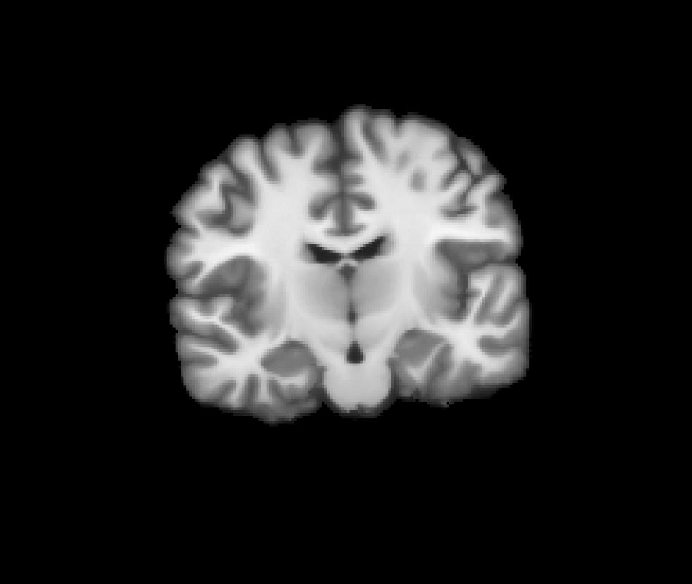
Coronal view of the target CVS space (norm.mgz) we want to resample to:
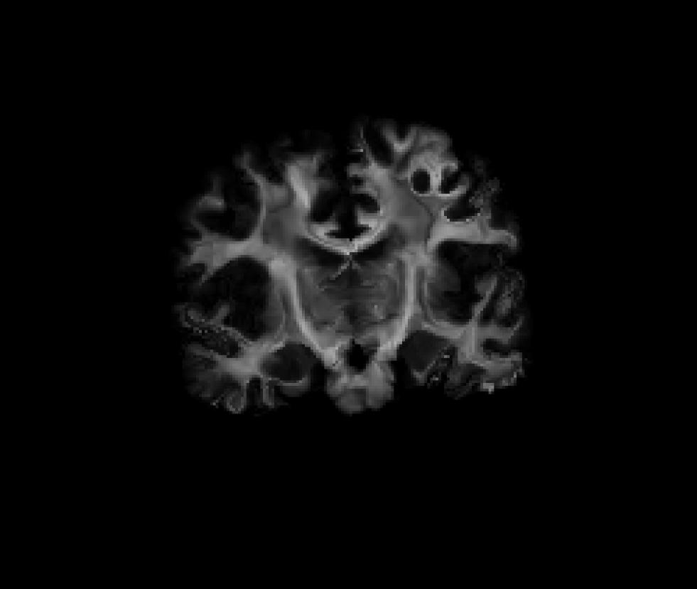
Coronal view of the masked fractional anisotropy volume after being resample to CVS space (fa-masked.ANAT+CVS-to-avg35.mgz):
Voxel-base Analysis / Group Analysis
Now that the DTI data for each subject is masked and normalized to a common space, we can performed analyses to determine
Assemble Data
In order to run the group analysis, 'mri_glmfit', you will need to first assemble your data in a particular manner. After having chosen on a coordinate space (i.e., CVS) where you want to do your analysis and have resampled all of your data into that space, you will need to create a single volume that stacks or concatenates all of the individual subject volumes. In the case of Freesurfer that would mean to create a volume with as many frames as the size of your input data set.
mkdir $TUTORIAL_DIR/GLM
set inputfiles = ($TUTORIAL_DIR/Diff???/dtrecon/fa-masked.ANAT+CVS-to-avg35.mgz)
echo $inputfiles
mri_concat --i $inputfiles --o $TUTORIAL_DIR/GLM/GroupAnalysis.fa-masked.CVS-to-avg35.Input.mgz
Note, the order of your image volumes on the data stack is important and it needs to match the order of entries in your fsgd file! In the above example, we first created an output directory for the group analysis (GLM). We then created a parameter called 'inputfiles' which contains all the names of the fractional anisotropy volumes that we want to inlcude in the study. The 'echo' command will print out the value of your parameter. It will give you a list of the file paths to each input volume, so that you can verify the order of the subject volumes matches the order of the entries in your fsgd file. The 'mri_concat' command is called to stack or concatenate the subjects' volumes into a multi-frame volume. We simply pass the command the input parameter 'inputfiles' containing the list of all the the fractional anisotropy volumes, and the file path and name of the desired output file (GroupAnalysis.fa-masked.CVS-to-avg35.Input.mgz).
For visualization purposes we will also create the average of the input images, so that we can overlay the group analysis results on top. We use the 'mri_average' command to create an average of the input images.
mri_average $inputfiles $TUTORIAL_DIR/GLM/Average.fa-masked.CVS-to-avg35.Input.mgz
When run, the 'mri_average' command produces a .mgz file, which is an average of the input volumes listed in the 'inputfiles' parameter.
For running the actual group analysis, we use the 'mri_glmfit' command. Besides the input data, we need to create an fsgd file and a contrast matrix, in order to describe what kind of analysis we are interested in.
FSGD text file (more info)
GroupDescriptorFile 1
Title Group Analysis
Class Male plus blue
Class Female circle green
SomeTag
Variables             Age
Input Diff001      Female 47
Input Diff002      Male   57
Input Diff003      Female 36
Input Diff004      Male   50
Input Diff005      Male   46
Input Diff006      Male   41
Input Diff007      Male   52
Input Diff008      Female 63
Input Diff009      Female 38
Input Diff010      Female 30
DefaultVariable Age
Contrast matrix file
0 0 .5 .5
mri_glmfit --y $TUTORIAL_DIR/GLM/GroupAnalysis.fa-masked.CVS-to-avg35.Input.mgz --fsgd group_analysis.fsgd dods\
           --C contrast.mtx --glmdir $TUTORIAL_DIR/GLM/gender_age.fa-masked.CVS-to-avg35.glmdir --mgz)
To see a script which could be used to do the two command steps above, take a look at the 'GroupAnalysis.csh' script on this page.
Now run mri_segstats: /// ARE WE DOING THIS?????????
mri_segstats \
  --seg $SUBJECTS_DIR/xxxxxxxxx.v4/mri/wmparc.mgz \
  --ctab $FREESURFER_HOME/FreeSurferColorLUT.txt \
  --id 251 --id 3021 --id 3024 --id 3030 --id 12 --id 4 \
  --i fa.anat.mgh --sum fa.stats
Click HERE to see the output. The CC has an average FA of about 0.75, gyral parcellations are about 0.4, the left putamen is 0.27, and the ventricle is 0.2. This is as expected because the CC is highly directional with no crossing fibers so we would expect the CC to have the highest FA. The gyral white matter is also directional but has fibers crossing in them, so one expects the FA to be lower than CC. The gray matter (putamen) is still lower. The ventricle has no fibers, so we expect it to have the lowest FA.
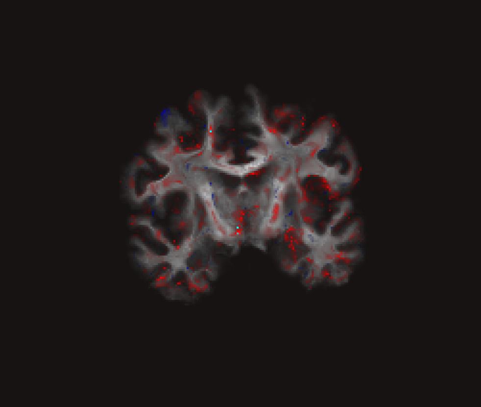
freeview –v $TUTORIAL_DIR/GLM/Average.fa-masked.CVS-to-avg35.Input.mgz \
            $TUTORIAL_DIR/GLM/gender_age.fa-masked.CVS-to-avg35.glmdir/contrast/sig.mgz:colormap=heat
Viewing:
Tractography
Using Trackvis to look at some of the results
Frequently Asked Questions
Q: Larger/Smaller gradient tables?
Q: Motion worse during diffusion scans?
Q: Inferences and assumptions being made with DTI data?
Q: What kind of research questions can be addressed with DTI data?
Q: Diffusion data collected on non-Siemens scanner?
Q: How to manually label tracks?
Q: Typical errors encountered during certains steps?
Acknowledgement
DTI tutorial scripts created by Lilla Zollei.
