|
Size: 18819
Comment:
|
Size: 18826
Comment:
|
| Deletions are marked like this. | Additions are marked like this. |
| Line 88: | Line 88: |
| {{attachment:label.jpg}} | {{attachment:label_coronal.jpg}} |
| Line 312: | Line 312: |
| {{attachment:spreadsheet.jpg}} | {{attachment:screenshot.jpg}} |
Anatomical ROI analysis
This tutorial gives a brief introduction to anatomical ROI analysis which includes working with label files, extracting ROI measures from the anatomical data, group statistics etc. Make sure you have set your SUBJECTS_DIR to correct location as
setenv TUTORIAL_DATA $FREESURFER_HOME/subjects/buckner_data/tutorial_subjs
setenv SUBJECTS_DIR $TUTORIAL_DATA/group_analysis_tutorial
cd $SUBJECTS_DIR
Relationship between segmentation, parcellation and LookUp Table (LUT)
In this exercise, you will examine a segmentation, parcellation, and color lookup table to understand how they are related.
Open the subject in tkmedit using the following command
tkmedit 004 orig.mgz -aux aparc+aseg.mgz \
  -seg aparc+aseg.mgz $FREESURFER_HOME/FreeSurferColorLUT.txt
Open another terminal to load the subject in tksurfer, using the following command.
tksurfer 004 lh inflated -annot aparc.annot
Finally, run the following command to display the contents of LUT
less $FREESURFER_HOME/FreeSurferColorLUT.txt
You can hit the 'Page Up' and 'Page Down' buttons to see the rest of the file. Or click here to view the contents of the file.
Things to do -- Navigating between tkmedit and LUT:
- Click on a point on the image loaded in tkmedit.
- See the structure name in the tkmedit Tools window (under the Cursor section).
- Look at the Aux (aparc+aseg.mgz) value in the tkmedit Tools window. For example, it may say 1024.
- Find that value in the LUT, which you have opened using the command mentioned above.
- Verify that it is the same structure as listed in tkmedit.
Things to do -- Navigating between tksurfer, tkmedit and LUT:
- Click on a point in tksurfer in the superior temporal gyrus. If you don't know it's location, you can hover over the different areas to see their label underneath the Mouse section of the Tools window.
- Note that the name displayed in the tksurfer Tools window does not have lh or rh in it. This is because you loaded only one hemisphere.
In tksurfer, click on the Save Point button

In tkmedit, click on Goto Point button
 , which takes the cursor to the ROI. Zoom in to see the cursor.
 - Verify the structure name in the tkmedit Tools window. Note that it DOES have an lh or rh in it.
- The Aux (aparc+aseg.mgz) value should be 1030.
- In FreeSurferColorLUT.txt, verify that 1030 is ctx-lh-superiortemporal
Label files
This section gives the details of commands to load an existing label file in text editor, tkmedit, and tksurfer.
To map a label, such a lh.BA45.label, from the fsaverage subject to a target subject, run
cd $SUBJECTS_DIR
mri_label2label \
  --srcsubject fsaverage \
  --srclabel fsaverage/label/lh.BA45.label \
  --trgsubject 004 \
  --trglabel 004/label/lh.BA45.label \
  --hemi lh \
  --regmethod surface
And then to look at the contents of that newly created label file, run
less 004/label/lh.BA45.label
To load the label in tkmedit, first load the subject you want to work on, in tkmedit.
tkmedit 004 orig.mgz
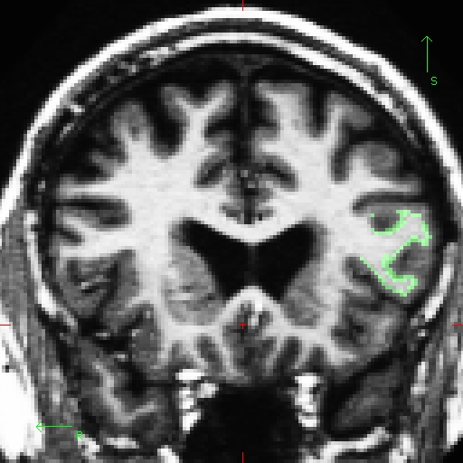
Then on the menu bar at the top of tkmedit tools window, go to File --> Label --> Load Label --> Browse --> lh.BA45.label and hit 'OK' in both windows. The label is visible in coronal slice 153.

This label can be edited when the Select Voxels button is chosen. Use the middle mouse button to add to the label. Use the right mouse button to delete from the label. If this was your own subject, you would want to make sure you save your edits by going to File --> Label --> Save Label but it's not necessary for this tutorial.
To load the label in tksurfer, first load the subject.
tksurfer 004 lh inflated
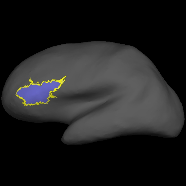
On the menu bar at the top of tksurfer tools window, go to File --> Label --> Load Label --> Browse --> lh.BA45.label

Information on how to create and edit labels in tksurfer can be found on this wiki.
Individual Stats files
During the normal FreeSurfer processing stream, via the recon-all script, (a freesurfer tutorial is available.) some statistical output files are generated. They are kept in each subjects' stats/ subdirectory and are generated for the subcortical segmentation (aseg) and the cortical parcellation (aparc). These tables include information on each labeled region for the individual subject.
aseg.stats
The statistical output from the subcortical segmentation, called aseg.stats, is a regular text file and will contain the volumes of specific structures. For example, you can obtain information such as the volume of left hippocampus and its mean intensity from this file.
cd $SUBJECTS_DIR/004/stats
less aseg.stats
At the head of the text file there will be information about the command that was run, the version used, the user who ran it and a time stamp. Following this there is information about the volume of the entire brain. This shows the number of voxels in the brainmask (BrainMaskNVox), the volume of the brainmask (BrainMaskVol), the number of voxels in the brainseg (BrainSegNVox), the volume of the brainseg (BrainSegVol), and the intracranial volume (ICV). This part of the file also tells us that the brainmask.mgz volume is being used as BrainMask (BrainMaskFile mri/brainmask.mgz) and the aseg.mgz segmentation is being used as the SegVol (SegVolFile mri/aseg.mgz). The number of voxels and the volumes should be the same for this subject, since this part of the file also tells us that the voxel volume is 1 mm3 (VoxelVolume_mm3 1) - and volume is measured in mm3.
The next section of this file defines the column headers, field name, and units for the rest of the table. We can expect to see the Segmentation Id, Number of Voxels, Volume, Structure Name, Intensity normMean, Intensity normStdDev, Intensity normMin, Intensity normMax, and Intensity normRange for each entry in the table.
The remainder of the table shows this information for all the structures that are labeled in the aseg.
# Title Segmentation Statistics
#
# generating_program mri_segstats
# cvs_version $Id: mri_segstats.c,v 1.33.2.5 2009/02/11 22:38:51 nicks Exp $
# cmdline mri_segstats --seg mri/aseg.mgz --sum stats/aseg.stats --pv mri/norm.mgz --excludeid 0 --brain-vol-from-seg --brainmask mri/brainmask.mgz --in mri/norm.mgz --in-intensity-name norm --in-intensity-units MR --etiv --subject 004 --surf-wm-vol --ctab /usr/local/freesurfer/stable4/ASegStatsLUT.txt
# sysname  Linux
# hostname compute-0-76.local
# machine  x86_64
# user     FS-user
# anatomy_type volume
#
# SUBJECTS_DIR /autofs/space/birn_045/users/BWH/buckner_data/group_study_fs4.3.0
# subjectname 004
# BrainMaskFile  mri/brainmask.mgz
# BrainMaskFileTimeStamp  2009/08/28 15:24:37
# Measure BrainMask, BrainMaskNVox, Number of Brain Mask Voxels, 1750419, unitless
# Measure BrainMask, BrainMaskVol, Brain Mask Volume, 1750419.000000, mm^3
# Measure BrainSegNotVent, BrainSegVolNotVent, Brain Segmentation Volume Without Ventricles, 1174751.000000, mm^3
# Measure BrainSeg, BrainSegNVox, Number of Brain Segmentation Voxels, 1234608, unitless
# Measure BrainSeg, BrainSegVol, Brain Segmentation Volume, 1234608.000000, mm^3
# Measure IntraCranialVol, ICV, Intracranial Volume, 1792580.562856, mm^3
# SegVolFile mri/aseg.mgz
# SegVolFileTimeStamp  2009/08/28 20:34:21
# ColorTable /usr/local/freesurfer/stable4/ASegStatsLUT.txt
# ColorTableTimeStamp 2009/08/23 07:21:06
# InVolFile  mri/norm.mgz
# InVolFileTimeStamp  2009/08/28 15:53:33
# InVolFrame 0
# PVVolFile  mri/norm.mgz
# PVVolFileTimeStamp  2009/08/28 15:53:33
# surface-based-volume mm3 lh-cerebral-white-matter 257166.312500
# surface-based-volume mm3 rh-cerebral-white-matter 258144.406250
# surface-based-volume mm3 tot-cerebral-white-matter 515310.718750
# ExcludeSegId 0
# VoxelVolume_mm3 1
-
-
-
# TableCol  1 ColHeader Index
# TableCol  1 FieldName Index
# TableCol  1 Units     NA
# TableCol  2 ColHeader SegId
# TableCol  2 FieldName Segmentation Id
# TableCol  2 Units     NA
# TableCol  3 ColHeader NVoxels
# TableCol  3 FieldName Number of Voxels
# TableCol  3 Units     unitless
# TableCol  4 ColHeader Volume_mm3
# TableCol  4 FieldName Volume
# TableCol  4 Units     mm^3
# TableCol  5 ColHeader StructName
# TableCol  5 FieldName Structure Name
# TableCol  5 Units     NA
-
-
-
# ColHeaders  Index SegId NVoxels Volume_mm3 StructName normMean normStdDev normMin normMax normRange
  1   2    219085   219085.0  Left-Cerebral-White-Matter       103.8966     9.6685    29.0000   175.0000   146.0000
  2   3    250309   250309.0  Left-Cerebral-Cortex              68.3985    10.8942     0.0000   138.0000   138.0000
  3   4     31187    31187.0  Left-Lateral-Ventricle            21.1173    10.2779     6.0000    97.0000    91.0000
  4   5      1232     1232.0  Left-Inf-Lat-Vent                 36.2831    12.5401    13.0000    87.0000    74.0000
  5   7     13596    13596.0  Left-Cerebellum-White-Matter      87.2863     7.6238    41.0000   122.0000    81.0000
  6   8     47867    47867.0  Left-Cerebellum-Cortex            60.4962     9.4270    23.0000    97.0000    74.0000
-
-
-
aparc.stats
The statistical output from the cortical parcellation, called lh.aparc.stats and rh.aparc.stats, is a regular text file and will contain the thickness of specific structures. For example, you can obtain information such as, how big is left superior temporal gyrus and its average thickness from this file.
cd $SUBJECTS_DIR/004/stats
less lh.aparc.stats
At the head of the text file there will be information about the command that was run, the version used, the user who ran it and a time stamp. Following this there is information about the volume of the entire brain. This shows the number of vertices in the cortex (NumVert), and the surface area of the cortex (SurfArea). This part of the file also tells us that the lh.aparc.annot is being used as the annotation file (AnnotationFile ../label/lh.aparc.annot).
The next section of this file defines the column headers, field name, and units for the rest of the table. We can expect to see the Structure Name, Number of Vertices, Surface Area, Gray Matter Volume, Average Thickness, Thickness StDev, Integrated Rectified Mean Curvature, Integrated Rectified Gaussian Curvature, Folding Index and Intrinsic Curvature Index for each entry in the table.
The remainder of the table shows this information for all the structures that are labeled in the aparc.
# Table of FreeSurfer cortical parcellation anatomical statistics
#
# CreationTime 2009/08/29-08:12:02-GMT
# generating_program mris_anatomical_stats
# cvs_version $Id: mris_anatomical_stats.c,v 1.54.2.7 2009/06/08 23:45:06 nicks Exp $
# mrisurf.c-cvs_version $Id: mrisurf.c,v 1.557.2.19 2009/08/05 22:10:21 nicks Exp $
# cmdline mris_anatomical_stats -mgz -f ../stats/lh.aparc.stats -b -a ../label/lh.aparc.annot -c ../label/aparc.annot.ctab 004 lh
# sysname  Linux
# hostname compute-0-83.local
# machine  x86_64
# user     FS-user
#
# SUBJECTS_DIR /autofs/space/birn_045/users/BWH/buckner_data/group_study_fs4.3.0
# anatomy_type surface
# subjectname 004
# hemi lh
# AnnotationFile ../label/lh.aparc.annot
# AnnotationFileTimeStamp 2009/08/29 04:11:56
# Measure Cortex, NumVert, Number of Vertices, 151235, unitless
# Measure Cortex, SurfArea, Surface Area,  100717, mm^2
-
-
-
# TableCol  1 ColHeader StructName
# TableCol  1 FieldName Structure Name
# TableCol  1 Units     NA
# TableCol  2 ColHeader NumVert
# TableCol  2 FieldName Number of Vertices
# TableCol  2 Units     unitless
# TableCol  3 ColHeader SurfArea
# TableCol  3 FieldName Surface Area
# TableCol  3 Units     mm^2
# TableCol  4 ColHeader GrayVol
# TableCol  4 FieldName Gray Matter Volume
# TableCol  4 Units     mm^3
# TableCol  5 ColHeader ThickAvg
# TableCol  5 FieldName Average Thickness
# TableCol  5 Units     mm
-
-
-
# ColHeaders StructName NumVert SurfArea GrayVol ThickAvg ThickStd MeanCurv GausCurv FoldInd CurvInd
unknown                                 10290   6406   7172  1.077 1.553     0.117     0.209     1036   124.5
bankssts                                 1409    973   2233  2.249 0.503     0.129     0.048       17     2.9
caudalanteriorcingulate                  1272    841   2523  2.647 0.792     0.163     0.084       36     4.2
caudalmiddlefrontal                      3361   2245   6597  2.579 0.581     0.140     0.050       42     7.0
cuneus                                   2423   1540   3093  1.819 0.393     0.167     0.074       46     6.6
entorhinal                                620    412   1814  3.190 0.648     0.145     0.066       11     1.8
-
-
-
Group stats files
This section will run you through using the stats directory in the subjects to perform group stats of certain structures that may be of interest to your study. The following commands will help you combine the data of the subjects you are analyzing into one table that will be easily read into a spreadsheet program. We have considered 6 subjects as examples (004, 021, 040, 067, 080, 092) in the following sections.
Set your SUBJECTS_DIR to the path where you have your subjects to be analyzed.
setenv SUBJECTS_DIR $TUTORIAL_DATA/group_analysis_tutorial
cd $SUBJECTS_DIR
Table of segmentation volumes
This section explains how to create a table of segmentation volumes using the 6 subjects mentioned above.
asegstats2table --subjects 004 021 040 067 080 092 \
  --segno 11 17 18 \
  --tablefile aseg.vol.table
where 11, 17 and 18 correspond to the segmentation label of left caudate, left hippocampus and left amygdala respectively. You can get the segmentation labels and the corresponding subcortical structures using the following command:
less $FREESURFER_HOME/FreeSurferColorLUT.txt
For tutorial purposes, click here to view the contents of the file.
The file aseg.vol.table is your output - a text file consisting of the subjects mentioned in the command above and the values for the structures requested. The information in this text file is formatted so it can be easily imported into a spreadsheet program. If you do the ls command, you should see that the text file aseg.vol.table has been created. To see what the file looks like, do:
less aseg.vol.table
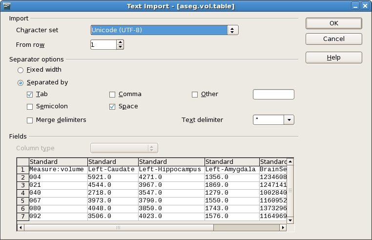
After running the asegstats2table command, to load the resulting table into a spreadsheet, run
oocalc aseg.vol.table
and then select Space in the Separated by menu.

Note: the oocalc command is meant to be run on a Linux machine. Mac users could install OpenOffice 3.0 to open the table in a spreadsheet and run the command
/Applications/OpenOffice.org.app/Contents/MacOS/scalc aseg.vol.table
In the table, the first cell is volume indicating that the measure is a volume in mm3. In addition to segmentations, you can also get IntraCranialVol (ICV) and BrainSegVol into the table.
About the subject IDs, you'll notice that in the examples we've considered here, each subject is a 3 digit number. Therefore oocalc thinks it is a number and removes leading 0s. This is an oocalc issue but probably it would not happen if subject names had characters in them instead of integers.
Table of segmentation mean intensities
Purpose of this section is to demonstrate how you can change what measure you collect for your spreadsheet from volume to mean intensity using the asegstats2table command.
asegstats2table \
  --subjects 004 021 040 067 080 092 \
  --segno 11 17 18 \
  --meas mean \
  --tablefile aseg.mean-intensity.table
Things to do:
- You can load the table into a spreadsheet as explained in the previous section.
Refer to the file FreeSurferColorLUT.txt for the segmentation labels and the corresponding subcortical structures.
less $FREESURFER_HOME/FreeSurferColorLUT.txt
For tutorial purposes, click here to view the contents of the file.
Table of white matter parcellation volumes
The purpose of this section is to show how you can change which segmentation atlas you get stats from (and thus which structures):
asegstats2table \
  --subjects 004 021 040 067 080 092 \
  --segno 3007 3021 3022 4022 \
  --stats wmparc.stats \
  --tablefile wmparc.vol.table
Things to do:
- You can load the table into a spreadsheet.
Refer to the file FreeSurferColorLUT.txt for the segmentation labels and the corresponding subcortical structures.
less $FREESURFER_HOME/FreeSurferColorLUT.txt
For tutorial purposes, click here to view the contents of the file
Table of the surface area of each cortical parcellation in the Desikan atlas
This section explains how to create a table of the surface area of each cortical parcellation in the Desikan atlas (surface area is the default measure).
aparcstats2table --hemi lh \
  --subjects 004 021 040 067 080 092 \
  --tablefile lh.aparc.area.table
You can now load the resulting table into a spreadsheet.
Table of the average thickness of each cortical parcellation in the Destrieux atlas
The purpose of this section is to show how to change the summary measure and the parcellation atlas.
aparcstats2table --hemi lh \
  --subjects 004 021 040 067 080 092 \
  --meas thickness \
  --parc aparc.a2005s \
  --tablefile lh.aparc.a2005.thickness.table
You can now load the resulting table into a spreadsheet.
