Back to Top Tutorial Page
Back to Multimodal Top
Other multimodal tutorials: A. Multimodal Registration, C. Surface-based Group fMRI Analysis, D. Individual DTI Integration
The purpose of this tutorial is to get you acquainted with the concepts need to perform fMRI integration in FreeSurfer by interacting with the data from an individual subject. You will not learn how to perform fMRI analysis here; that knowledge is already assumed. This tutorial also does not assume any particular directory strucutre (as would happen in FS-FAST). This tutorial makes use of data from the Functional Biomedical Informatics Research Network (fBIRN, www.nbirn.net).
Contents
fMRI Basics
In fMRI, stimuli are presented to a subject, which creates a BOLD hemodynamic response function (HRF) in certain areas of the brain. The analysis is performed by first performing motion correction, then correlating each voxel's time course with the stimulus schedule convolved with an assumed HRF shape. The result is an estimate of the HRF amplitude for each condition at each voxel, contrasts of the HRF amplitudes of various conditions, the variance of this contrast, and some measure of the signficance (eg, p, t, F, or z) map. All these maps are aligned with the motion correction template, which should be used as the registration tempate.
This Data Set
All the commands in this section should be run from this directory
setenv TUTORIAL_DATA $FREESURFER_HOME/subjects/buckner_data/tutorial_subjs
setenv SUBJECTS_DIR $TUTORIAL_DATA
cd $TUTORIAL_DATA/multimodal/fmri/fbirn-101
This is one of 5 subjects from the fBIRN Phase I acquisition. They are fbirn-10?, where "?" is 1, 3, 4, 5, 6 (note that #2 is missing). Each has a FreeSurfer reconstruction by the name fbirn-anat-10?.v4. This tutorial will only deal with fbirn-101 (but you can run the same commands on any of them).
The data are the results from a sesorimotor paradigm (flashing checkerboard, audible tone, and finger tapping). The raw fMRI data were motion corrected but not smoothed. Each subject has four volumes:
template.nii - motion correction template
ces.nii - contrast effect size
cesvar.nii - variance of contrast effect size
sig.nii - signed signifiance of contrast (-log10(p))
The contrast is the contrast between the ON and the OFF (ie, a comparison against baseline). The sig.nii volume has signed -log10(p) values. So, if the p-value = .01, -log10(p) = 2. If the contrast was positive, then the value would be +2, if negative (ie, ON<OFF), then the value would be -2.
Check Registration
First (and always), check the registration (see the Registration Tutorial for more information).
tkregister2 --mov template.nii \
  --reg bb.register.dat --surf
This registration should already be good, so there is no need to make any modifications.
View sig map on anatomical volume
tkmedit fbirn-anat-101.v4 orig.mgz -aux brain.mgz -seg aparc+aseg.mgz \
  -overlay sig.nii -reg bb.register.dat -fthresh 2 -fmax 4
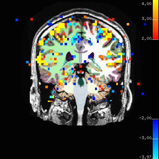
Notes:
ON>OFF is red/yellow
ON<OFF is blue/cyan
- Notice activation in motor, auditory, and visual regions.
- As you click on the volume loaded in tkmedit, you will see the "Functional value" field in the Tools window change as well as the "Sgmtn label"
Note that the -fthresh flag is given a value of 2 in the command line above. fthresh is the functional value of the voxel which is the threshold value for a voxel to show up on the overlay.
- Functional value is the -log 10(p value) which makes the p-value here 0.01
- Also note that areas that are not above threshold will still have non-zero functional values
Things to do:
You can turn the overlay ON or OFF using the 'Show Functional Overlay' tool button on the tkmedit tools window

To understand and experiment with this image further, go to View --> Configure --> Functional Overlay, on the menu bar at the top of tools window. You'll see an interface which looks as follows.
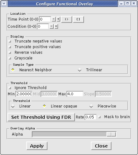
- Try changing the minimum and maximum threshold values, which are currently set at 2 and 4 respectively, hit 'Enter' and click on 'Apply'.
View sig map on left hemisphere
Before you can view the fMRI data on the surface, you must resample the data onto the surface:
mri_vol2surf --mov sig.nii \
    --reg bb.register.dat \
    --projfrac 0.5 --interp nearest \
    --hemi lh --o lh.sig.mgh
Notes:
- The "moveable" is the signficance map (which is in line with the template.nii used for registration).
- "--projfrac 0.5" indicates that the significance should be sampled half way between the white and pial surfaces.
- "--interp nearest" means use nearest neighbor interpolation (good for sig).
The output is lh.sig.mgh the significance sampled onto the left hemisphere. It has the same size as any other surface overlay for this subject, eg, lh.thickness. To see it's dimensions, run:
mri_info lh.sig.mgh
You will see "dimensions: 54707 x 1 x 3", indicating that there are 54707 "columns" (ie, vertices), 1 "row", and 3 "slices". Multiplying them together gives 164121 which is the number of vertices in the surface.
tksurfer fbirn-anat-101.v4 lh inflated -annot aparc \
  -overlay lh.sig.mgh
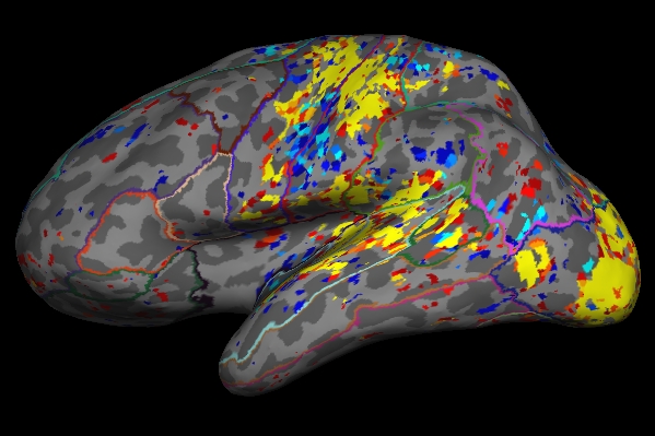
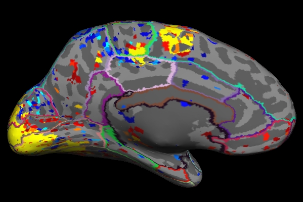
Things to Note:
- As mentioned in the previous section, the example we've considered here is the result from administering sensorimotor task. The activation can be seen in the corresponding regions, Auditory cortex (Temporal lobe), Visual cortex (Occipital lobe), Motor cortex (Parietal lobe).
- Click on a point on the surface and notice the label change.
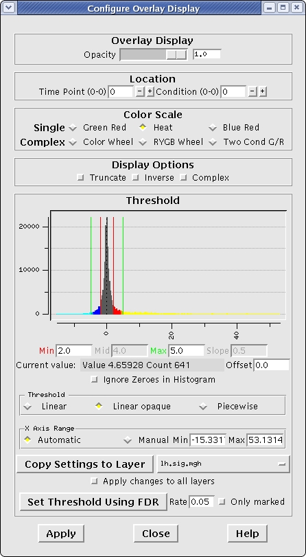
Change the min and max threshold values and notice the overlay changes. To do this go to, View --> Configure --> Overlay, on the menu bar at the top of tools window. This brings up an interface which looks as follows. The min and max threshold values are currently set to 2 and 5 respectively.
ROI Analysis without a Functional Constraint
In this section, we will compute the average HRF contrast (ces) in some ROIs. First, we need to resample the ces.nii volume into the individual's anatomical space:
mri_vol2vol --mov ces.nii \
    --reg bb.register.dat \
    --fstarg --interp nearest \
    --o ces.anat.bb.mgh
Notes:
- "--fstarg" means to sample the data into the anatomical space
- Nearest-neighbor (--interp nearest) because we will average within each ROI so we do not want averaging from interpolation.
The output is ces.anat.bb.mgh. Look at it's dimensions:
mri_info ces.anat.bb.mgh
Note that it is 256x256x256 with each voxel being 1mm isotropic. This is the same size as the FreeSurfer anatomical.
Now run the segmentation statistics:
mri_segstats \
   --seg $SUBJECTS_DIR/fbirn-anat-101.v4/mri/aparc+aseg.mgz \
   --ctab $FREESURFER_HOME/FreeSurferColorLUT.txt \
   --id 1021 --id 1022 --id 1030  --id 17 \
   --i ces.anat.bb.mgh --sum ces.bb.stats
Notes:
- The subject's own aparc+aseg.mgz is used
Segmentation names come from the LUT. Click here to view the contents of the LUT file.
- Report on only 4 segmentations are requested (1021=ctx-lh-pericalcarine, 1022=ctx-lh-postcentral, 1030=ctx-lh-superiortemporal, and 17=Left-Hippocampus). The first three are related to the paradigm.
- The input is ces.anat.bb.mgh
Look at the output ces.bb.stats in a text viewer (or click here). It has a format very similar to the aseg.stats file in each subject's stats directory. The "Mean" here is the average HRF amplitude in the given ROI in raw MR units. Eg, the average HRF amplitude in ctx-lh-pericalcarine is 112.9913. Note that the volume is 2586.0 mm3; this is the volume of the ctx-lh-pericalcarine segmentation.
ROI Analysis with an Unsigned Functional Constraint
In this section, we will compute the average HRF contrast (ces) in anatomical ROIs constrained by functional activation. First, we need to resample the sig.nii volume into the individual's anatomical space:
mri_vol2vol --mov sig.nii \
    --reg bb.register.dat \
    --fstarg --interp nearest \
    --o sig.anat.bb.mgh
Notes:
- "--fstarg" means to sample the data into the anatomical space
- Nearest-neighbor (--interp nearest) because this is a significance volume.
Now run the segmentation statistics with the functional constraint:
mri_segstats \
   --seg $SUBJECTS_DIR/fbirn-anat-101.v4/mri/aparc+aseg.mgz \
   --ctab $FREESURFER_HOME/FreeSurferColorLUT.txt \
   --id 1021 --id 1022 --id 1030  --id 17 \
   --i ces.anat.bb.mgh --sum ces.abs-masked.bb.stats \
   --mask sig.anat.bb.mgh --maskthresh 2 --masksign abs
Notes:
- The mask is the signficance map
The threshold is 2 (p<.01)
- "--masksign abs" means to use any voxel that exceeds threshold regardless of its sign.
Look at the output ces.abs-masked.bb.stats in a text viewer (or click here). The "Mean" for ctx-lh-pericalcarine is now 181.3009, an increase of 60%. The increase is because all of those voxels that did not have any signal were excluded from the ROI average. The volume is now 1512.0 mm3, meaning that 58% (1512.0/2586.0) of the ROI is above thershold.
ROI Analysis with a Positive Functional Constraint
In this section, we will compute the average HRF contrast (ces) in anatomical ROIs constrained by positive functional activation only. Run the segmentation statistics with the functional constraint:
mri_segstats \
   --seg $SUBJECTS_DIR/fbirn-anat-101.v4/mri/aparc+aseg.mgz \
   --ctab $FREESURFER_HOME/FreeSurferColorLUT.txt \
   --id 1021 --id 1022 --id 1030  --id 17 \
   --i ces.anat.bb.mgh --sum ces.pos-masked.bb.stats \
   --mask sig.anat.bb.mgh --maskthresh 2 --masksign pos
Notes:
- "--masksign pos" means to use any voxel that exceeds threshold and has a positive sign.
Look at the output ces.pos-masked.bb.stats in a text viewer (or click here). The "Mean" for ctx-lh-pericalcarine is now 198.2415, an increase of 10% over the unsigned case. The increase is because some of the voxels in the unsigned case are negative and so reduce the ROI average. Note that the volume has dropped to 1408.0 mm3 because the negative voxels have been removed. Note: in this case the Mean will always be positive because we have constrained it that way!
Other multimodal tutorials: A. Multimodal Registration, C. Surface-based Group fMRI Analysis, D. Individual DTI Integration
