| Deletions are marked like this. | Additions are marked like this. |
| Line 31: | Line 31: |
|
In the Scan Setting menu, ensure the “with Turntable” box is checked. The alignment mode using markers is used instead of “Turntable Coded Targets” because tissue can easily cover turtable targets affecting point-cloud registration. Tissue should not slide on the turtable surface, sliding can be especially present when scanning the medial wall and can be helped by lowering the turtable speed, we recommend a speed setting of 3, and gently patting the tissue with a linen towel to remove some excess fixative. When using the handheld mode, we highly recommend also using markers which vastly improve scanning speed and user experience. Turntable steps determine how many scans will be acquired and stitched. More steps can lead to a higher resolution surface but can increase scan time. There are also diminishing returns with setting too many turtable steps. We recommend setting turntable steps to 36, which we consider a good balance between acquisition time and scan quality. |
In the Scan Setting menu, ensure the “with Turntable” box is checked. The alignment mode using markers is used instead of “Turntable Coded Targets” because tissue can easily cover turntable targets affecting point-cloud registration. Tissue should not slide on the turntable surface, sliding can be especially present when scanning the medial wall and can be helped by lowering the turntable speed, we recommend a speed setting of 3, and gently patting the tissue with a linen towel to remove some excess fixative. When using the handheld mode, we highly recommend also using markers which vastly improve scanning speed and user experience. Turntable steps determine how many scans will be acquired and stitched. More steps can lead to a higher resolution surface but can increase scan time. There are also diminishing returns with setting too many turntable steps. We recommend setting turntable steps to 36, which we consider a good balance between acquisition time and scan quality. |
| Line 45: | Line 45: |
| Post sectioning of the cerebellum, we obtain a surface scan of the specimen before then secitoning it into slabs for photography. We place a glass sheet atop to protect the turntable and ease cleanup. The glass sheet contains markers that be used for tracking. The specimen is placed in the middle of the turntable so that the scanner gets the best view of the sample as it rotates. Occluding the turntable markers will also affect the stitching of scans if the scan is set to “Turntable Coded Targets.” When using custom markers howerver, which we recommend, the turtable targets should be covered completely. When using custom markers in either fixed or handheld mode, make sure the specimen is not covering any markers on the glass sheet. | Post sectioning of the cerebellum, we obtain a surface scan of the specimen before then sectioning it into slabs for photography. We place a glass sheet atop to protect the turntable and ease cleanup. The glass sheet contains markers that be used for tracking. The specimen is placed in the middle of the turntable so that the scanner gets the best view of the sample as it rotates. Occluding the turntable markers will also affect the stitching of scans if the scan is set to “Turntable Coded Targets.” When using custom markers however, which we recommend, the turntable targets should be covered completely. When using custom markers in either fixed or handheld mode, make sure the specimen is not covering any markers on the glass sheet. |
| Line 56: | Line 56: |
| Handheld mode can be particularly useful for fresh tissue, since it connot maintain its shape or be flipped for two-sided scans because of deformation. In this mode, a transparent surface can be used to scan both sides of the sample without having to shift the easily deformable tissue. | Handheld mode can be particularly useful for fresh tissue, since it cannot maintain its shape or be flipped for two-sided scans because of deformation. In this mode, a transparent surface can be used to scan both sides of the sample without having to shift the easily deformable tissue. |
| Line 69: | Line 69: |
|
Use the preview window to check exposure, areas that are overexposed will appear red. A good exposure will show some red areas but too many, see bewlow for a referecne of a good exposure. For specimens with particularly difficult lighting HDR mode can be used to better rended darker fearures. |
Use the preview window to check exposure, areas that are overexposed will appear red. A good exposure will show some red areas but too many, see below for a reference of a good exposure. For specimens with particularly difficult lighting HDR mode can be used to better render darker features. |
| Line 95: | Line 95: |
|
If you have two scanning sessions, there are a couple of ways the point-clouds can be registered, an automatic and manual method. Only use manual aligment if the automatic method fails. <<BR>> 1. Click the alignment icon and select both scanning sessions. Click the automatic alignment button at the top left of the screen. If the aligment fails, continue with the next steps. |
If you have two scanning sessions, there are a couple of ways the point-clouds can be registered, an automatic and manual method. Only use manual alignment if the automatic method fails. <<BR>> 1. Click the alignment icon and select both scanning sessions. Click the automatic alignment button at the top left of the screen. If the alignment fails, continue with the next steps. |
| Line 112: | Line 112: |
| When acquiring the mesh, the sides of the sample are critical for proper point cloud alignment. Poorly captured sides will lead to innacurate alignments between scans, which will cause issues in the final reconstruciton. The following example shows a handheld scan where the sides of the tissue were not acquired, resulting in a flatter/thinner appearance which will negatevely affect the quality of the final reconstruction. | When acquiring the mesh, the sides of the sample are critical for proper point cloud alignment. Poorly captured sides will lead to inaccurate alignments between scans, which will cause issues in the final reconstruction. The following example shows a handheld scan where the sides of the tissue were not acquired, resulting in a flatter/thinner appearance which will negatively affect the quality of the final reconstruction. |
| Line 123: | Line 123: |
| The following guidelines should be followed when prepararing slab images for optimal results. <<BR>> | The following guidelines should be followed when preparing slab images for optimal results. <<BR>> |
| Line 133: | Line 133: |
|
|
|
| Line 144: | Line 141: |
| Another example of difficult tissue placement can be the corpus callosum. In the following figure, we see a good example setup with high contrast for the background and good lighting. However, the placement of the corpus collosum on the rightmost slab is incorrect, which will negatively affect volumetric estimates of the third ventricle. | Another example of difficult tissue placement can be the corpus callosum. In the following figure, we see a good example setup with high contrast for the background and good lighting. However, the placement of the corpus callosum on the rightmost slab is incorrect, which will negatively affect volumetric estimates of the third ventricle. |
| Line 159: | Line 156: |
| The optimal scenario is to have 4 points defined by fiducial markers with hihgly salient features. This enables our software to automatically recognize the fiducials, which minimizes human interaction, reducing time and maximizing reproducibility. We '''strongly''' recommend that you print these set fiducials and place them on the corners of the board. | The optimal scenario is to have 4 points defined by fiducial markers with highly salient features. This enables our software to automatically recognize the fiducials, which minimizes human interaction, reducing time and maximizing reproducibility. We '''strongly''' recommend that you print these set fiducials and place them on the corners of the board. |
| Line 179: | Line 176: |
| '''''Tip''''': It does not matter if slabs are not presented on a grid, as long as the distance between the fiducials is knwon. The software will draw digital rulers for your images later pixel-correction.<<BR>><<BR>> | '''''Tip''''': It does not matter if slabs are not presented on a grid, as long as the distance between the fiducials is known. The software will draw digital rulers for your images later pixel-correction.<<BR>><<BR>> |
| Line 186: | Line 183: |
| To install Freesurfer, follow the instructions on the Freesurfer website to download the latest stable release, note the tools in this tutorial are scheduled to be relesed in stable version 7.5: | To install Freesurfer, follow the instructions on the Freesurfer website to download the latest stable release, note the tools in this tutorial are scheduled to be released in stable version 7.5: |
| Line 197: | Line 194: |
| The photo reconstruction pipeline uses a nnUNet neural network model to segment the brain slabs to decreate the time involved in manualy segmenting photographs. When running '''dissection_photo_gui''' you must point to the directory where the model weights are stored. The model weights can be downloaded from the following link: | The photo reconstruction pipeline uses a nnUNet neural network model to segment the brain slabs to decrease the time involved in manually segmenting photographs. When running '''dissection_photo_gui''' you must point to the directory where the model weights are stored. The model weights can be downloaded from the following link: |
| Line 201: | Line 198: |
| After downloading, extract the files to a directory of your choice. It is recommended to store them in the following freesurfer directory, as it will be the default location our GUI uses. '''$FREESURFER_HOME_FSPYTHON/models/''' | After downloading, extract the files to a directory of your choice. It is recommended to store them in the following Freesurfer directory, as it will be the default location our GUI uses. '''$FREESURFER_HOME_FSPYTHON/models/''' |
| Line 205: | Line 202: |
| = Recommened Directory Structure = | = Recommended Directory Structure = |
| Line 214: | Line 211: |
| 1. connected_components - npz files showing the connected components for each image. | 1. connected_components - .npz files showing the connected components for each image. |
| Line 222: | Line 219: |
| The following guide will walk through the steps to preprocessing the brain slab images. This includes pixel correction, binarizing images, and selecting connected components. Make sure freesurfer is properly sourced, and you have downloaded the model weights before continuing with the tutorial. <<BR>> | The following guide will walk through the steps to preprocessing the brain slab images. This includes pixel correction, binarizing images, and selecting connected components. Make sure Freesurfer is properly sourced, and you have downloaded the model weights before continuing with the tutorial. <<BR>> |
| Line 243: | Line 240: |
| The dissection photo GUI performs all prepricessing tasks, including pixel correction, binarizing images, and selecting connected components. Before running the GUI, ensure these two enviroment variables are set if additional files are not in the default locations. | The dissection photo GUI performs all preprocessing tasks, including pixel correction, binarizing images, and selecting connected components. Before running the GUI, ensure these two environment variables are set if additional files are not in the default locations. |
| Line 249: | Line 246: |
|
To run the GUI, source freesurfer and use command '''dissection_photo_gui'''. <<BR>> == Retrospective Registration == Although less preferable, for images that do not have fiducials, we can still pixel-correct images using other references in the image, like a ruler, for each of the images. 1. Source the dev version of Freesurfer. 1. Organize your directory structure. 1. Run the retrospective registration command “retrospective_correction.” Select “Click to Start” on the first dialogue box. {{attachment:35_retrospectiveIntro.png||width="630",height="210"}} <<BR>> Select mode and indicate file paths. A new dialogue box (pictured below) will appear. Follow the directions as such: 1. Select the directory with the input images (the untouched sectioned brain images) by clicking the Choose Folder option. 1. Select the directory for the output images to be saved. As stated, this directory must already be created. 1. Select the mode that will be used for pixel correction. Select a mode that is compatible with your image setup. 2 points should be chosen if there is a single axis of ground truth measurement (i.e., One ruler in the image), and four should be chosen if there are two axes. {{attachment:36_retrospectiveDirectory.png||width="557",height="303"}} <<BR>> <<BR>> {{attachment:37_retrospectiveTissue.png||width="568",height="445"}} <<BR>> A new interactive window with your brain slabs and a “Ruler Length” option will be displayed. Click visible markers that provide ground truth measurement. Use these as the basis for your ruler Length, which should be entered in millimeters. Then, click register and complete the remaining images. The pixel-corrected images will then populate your output directory. Finally, save your subject’s registered images to your subject’s ‘deformed’ subdirectory. <<BR>><<BR>><<BR>> == Binarizing Images == Binary masks are created to only include the tissue slice and not include any cortex. Image editing software like GIMP can be used to create these binary masks. A combination of the thresholding and lasso tool is used to remove any non-slice tissue and the background. <<BR>><<BR>><<BR>> |
To run the GUI, source Freesurfer and use command '''dissection_photo_gui'''. <<BR>> == Pixel Correction == In the first menu of the '''dissection_photo_gui''' select the input directory with the unprocessed gross photographs. Photographs should be set in the order such that tissue slabs are seen in the order they were cut. Additionally select the output directory where the pixel-corrected images will be saved. Here we have the option to load an optimal calibration file if available to automate pixel correction. Select '''Go!''' when you have defined the required directories. <<BR>> {{attachment:35_dissection_photo_gui_screen_1.png||width="600",height="400"}} <<BR>> If a calibration file was used the next widow will display the pixel-corrected images for quality assurance purposes. Click '''Next''' to proceed assuring the images were corrected.<<BR>><<BR>> If no calibration file is provided the next window will be for the '''Retrospective Correction''' mode. Select the type of calibration, 2-point, 3-point, or 4-point, and its relevant dimensions in millimeters. The 2-point calibration is used when there is a single axis of ground truth measurement (i.e., One ruler in the image), and four should be chosen if there are two axes, as it will also correct for perspective. We can pan and zoom to make precise selection on the image. <<BR>> {{attachment:36_dissection_photo_gui_screen_2.png||width="600",height="400"}} <<BR>> {{attachment:37_dissection_photo_gui_screen_2_zoomed.png||width="600",height="400"}} <<BR>> After pixel correcting all images, click '''Proceed to Segmentation''' to continue to the next step.<<BR>> == Tissue Segmentation == After selecting an output directory for the masked images, our automatic segmentation tool will immediately start predicting a binary mask per each photograph. If a GPU is available all five folds of the model will be run which will slightly increase segmentation accuracy. After the first photograph is segmented by the model, the user can start cleaning the predicted binary masks. Here the user can pan and zoom like before, but can additionally use a brush tool to remove or add any pixels. Remove any non-slice tissue and the background. The opacity of the predicted mask can also be changed using the provided slider, or toggled using Ctrl+Z. <<BR>> {{attachment:38_dissection_photo_gui_screen_3_noseg.png||width="600",height="400"}} <<BR>> {{attachment:39_dissection_photo_gui_screen_3_seg.png||width="600",height="400"}} <<BR>> '''IMPORTANT''': The cortical surface should not be part of the masks, so the first (if photographed from the anterior side) or last slice (if photographed from the posterior side) should '''NOT''' be considered. You can either leave it out of the mask or ignore it when processing with the GUI. <<BR>> Once we are satisfied with the mask, click '''Next''' to proceed to the next image. After all images have been segmented and cleaned, click '''Proceed to CC''' to continue to the connected components step. <<BR>> |
| Line 279: | Line 272: |
|
This section covers how to use the connected components GUI to select brain slices. 1. Source the dev version of Freesurfer. 1. Run the fiducial calibration with the command “connected_components.” Following these directions, select the directory with the input images (the pixel-corrected deformed images). 1. Select the directory with the input masks created through GIMP. 1. Select the directory where you want the output masks saved. By clicking '''Click to Start''', you will land on the following interactive module. Input the directory destinations here. {{attachment:38_ccIntro.png||width="517",height="287"}} <<BR>> {{attachment:39_ccDirectory.png||width="560",height="328"}} <<BR>> By clicking '''Start Processing''', you will open a new interactive window displaying the deformed brain slab photographs. For each image, select slices in order by clicking and dragging to draw a box in a region of each individual slab in the photograph. After a box has been drawn in each individual slab, click '''Process Image '''to save the output .npy files. Make sure no boxes are overlapping. {{attachment:40_ccMain.png||width="575",height="453"}} <<BR>> Once a box is drawn over the tissue, the slab will be colored to show what is being included as a slice. {{attachment:41_ccBox.png||width="582",height="458"}} <<BR>> Above is an example of how to correctly draw the boxes within the brain slabs themselves. These boxes inform the GUI that the pixels connected to these slabs are all related. It is important that there is a disconnection between these slabs with some empty/black space between them so the GUI does not count two separate slabs as a single connected component. Additionally, note that the slabs are selected in the order they were cut. {{attachment:42_ccBoxLarge.png||width="579",height="457"}} <<BR>> Above is an example of how NOT to draw boxes for this GUI. Notice the occurrence of overlap between boxes and the inclusion of an abundance of black space. Try to keep the boxes drawn to small regions within the brain slabs themselves. '''IMPORTANT''': The cortical surface should not be part of the masks, so the first (if photographed from the anterior side) or last slice (if photographed from the posterior side) should '''NOT''' be considered. You can either leave it out of the mask or ignore it when processing with the unknown GUI. <<BR>><<BR>><<BR>> |
Like previous steps, select an output directory for the connected components masks. The connected components section of the GUI will display the masked and pixel-corrected photographs. Here the user will draw boxes around the tissue slabs in each photograph. The GUI will then save the connected components as .npy files. <<BR>> {{attachment:40_dissection_photo_gui_screen_4_tissue.png||width="600",height="400"}} <<BR>> For each image select slices in order, either anterior-posterior or posterior-anterior. Remain consistent of slice order on all photographs. Connected components are selected by clicking and dragging to draw a box in a region of each individual slab in the photograph. After a box has been drawn in each individual slab, click '''Next ''' to save the output .npy file and move to the next image. '''Tip''': Make sure no boxes are overlapping. Once a box is drawn over the tissue, the slab will be colored to show what is being included as one slice.<<BR>> {{attachment:41_dissection_photo_gui_screen_4_color.png||width="600",height="400"}} <<BR>> Above is an example of how to correctly draw the boxes within the brain slabs themselves. These boxes inform the GUI that the pixels connected to these slabs are all part of the same tissue slice. Note the box covers tissue from the temporal lobe as it can sometimes be disjoint from the rest of the slab. <<BR>> Below is an example of how not to draw boxes for this GUI. Notice the occurrence of overlap between boxes and the inclusion of an abundance of black space. Try to keep the boxes drawn to small regions within the brain slabs themselves as to not include any background pixels. <<BR>> {{attachment:42_dissection_photo_gui_screen_4_bad.png||width="600",height="400"}} <<BR>><<BR>> |
Photo Reconstruction Documentation
Contents
If you use these tools in your analysis, please cite:
* Machine learning of dissection photographs and surface scanning for quantitative 3D neuropathology. H Gazula, H Tregidgo, B Billot, Y Balbastre, J Williams Ramirez, R Herisse, LJ Deden-Binder, A Casamitjana, EJ Melief, CS Latimer, MD Kilgore, M Montine, E Robinson, E Blackburn, MS Marshall, TR Connors, DH Oakley, MP Frosh, SI Young, K Van Leemput, AV Dalca, B Fischl, CL Mac Donald, CD Keene, B Hyman, and JE Iglesias. Under revision.)
Click here for a video with an overview of the method
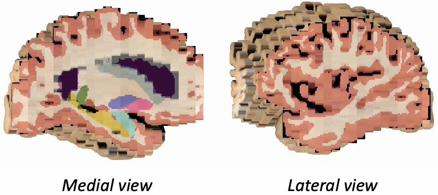
Purpose
This manual provides step-by-step instructions for using a 3D scanner on ex-vivo brain specimens, preparing tissue slabs for gross photography, and outlining the data processing pipeline to create a 3D reconstruction of brain slab images using the acquired scan as a reference surface.
Surface Scanning Protocol
This section covers the standard operating procedure for scanning fixed ex-vivo tissue specimens at Massachusetts General Hospital (MGH). We use an EinScan Pro HD scanner with the 'industrial pack,' which includes a turntable to automatically scan the specimen at multiple angles. A high quality surface scan is crucial for accurately reconstructing tissue slabs, as it serves as the reference for registering and deforming the slabs. Later sections will cover surface mesh quality assessments and tips to check scans.
Scanner Setup
To set up the turntable and scanner, we adjust the tripod ensuring a clear view of the full turntable plate. The scanner is placed approximately 45˚ and 8-10 inches from the turntable. If the turntable is unavailable, the SHINING3D software will guide the user on the appropriate scanner distance when using 'Handheld' mode. A later section covers some tips for scanning in handheld mode.
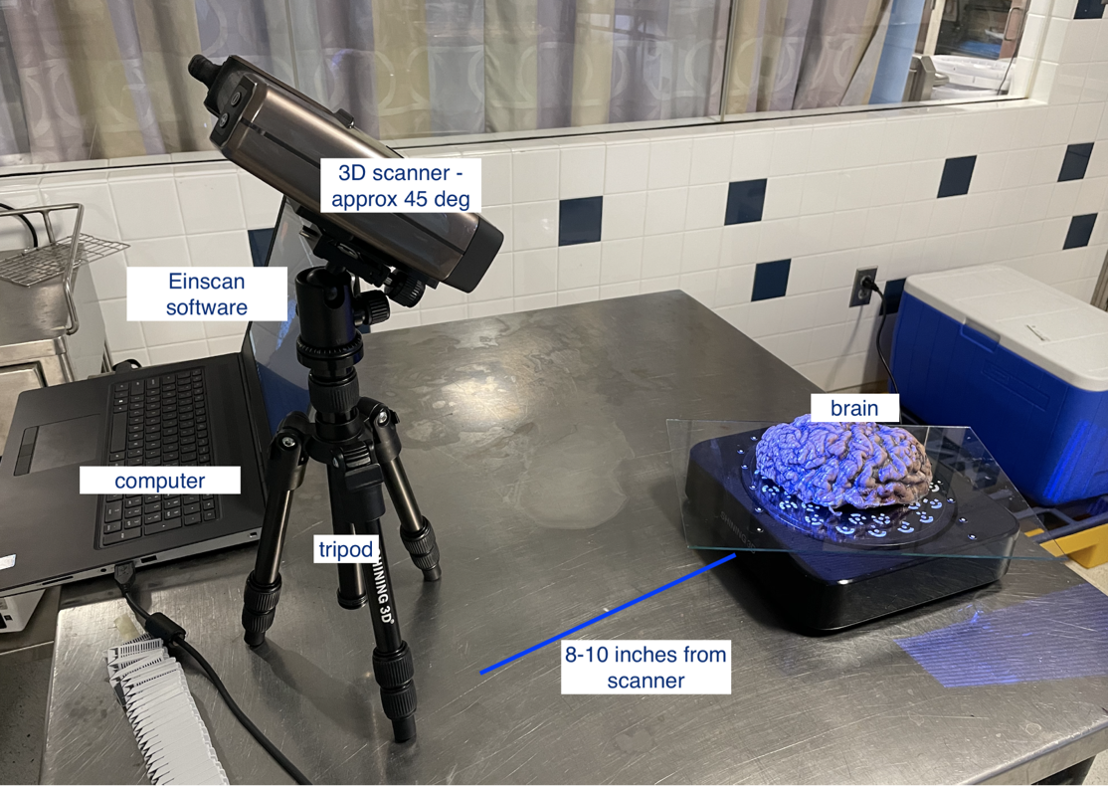
Scanner setup for turntable scan.
Next, launch the most up-to-date Shining3D software for the Einscan Pro HD. Software for all EinsScan 3D scanners can be found here einscan.com/support/download/. A menu will prompt a selection for the type of scan, fixed scan (using the turntable), handheld HD scan, or handheld rapid scan. Select “fixed scan” to use the turntable add-on and create a new “Non-texture Scan” project.
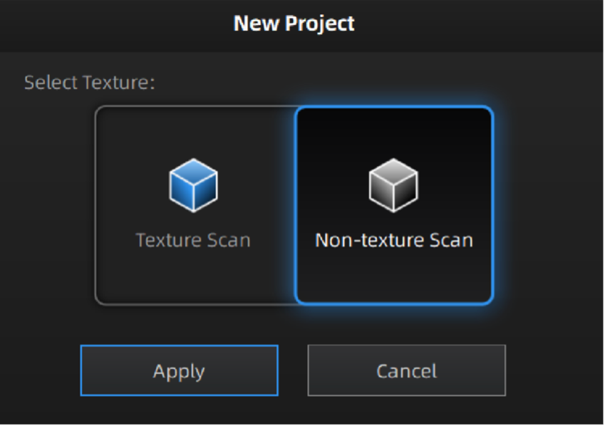
Texture settings prompt when creating a new project.
At this point, the main scan menu should be on the screen, where we can customize different parameters for scan acquisition. On the left-hand side of the screen, there is a preview of the scanner’s field of view.
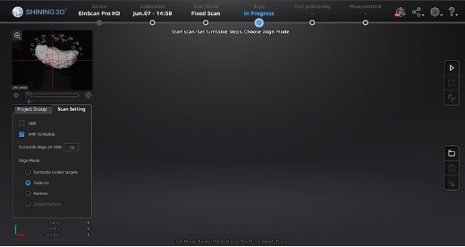
Main scan menu.
In the Scan Setting menu, ensure the “with Turntable” box is checked. The alignment mode using markers is used instead of “Turntable Coded Targets” because tissue can easily cover turntable targets affecting point-cloud registration. Tissue should not slide on the turntable surface, sliding can be especially present when scanning the medial wall and can be helped by lowering the turntable speed, we recommend a speed setting of 3, and gently patting the tissue with a linen towel to remove some excess fixative. When using the handheld mode, we highly recommend also using markers which vastly improve scanning speed and user experience.
Turntable steps determine how many scans will be acquired and stitched. More steps can lead to a higher resolution surface but can increase scan time. There are also diminishing returns with setting too many turntable steps. We recommend setting turntable steps to 36, which we consider a good balance between acquisition time and scan quality.
For handheld scans, we use the parameters:
- Texture: Non-texture scan
- Mode of alignment: hybrid
- Operation mode: classic (scanning speed: 15 fps)
- Resolution: high (0.5mm)
Sample Setup
Post sectioning of the cerebellum, we obtain a surface scan of the specimen before then sectioning it into slabs for photography. We place a glass sheet atop to protect the turntable and ease cleanup. The glass sheet contains markers that be used for tracking. The specimen is placed in the middle of the turntable so that the scanner gets the best view of the sample as it rotates. Occluding the turntable markers will also affect the stitching of scans if the scan is set to “Turntable Coded Targets.” When using custom markers however, which we recommend, the turntable targets should be covered completely. When using custom markers in either fixed or handheld mode, make sure the specimen is not covering any markers on the glass sheet.
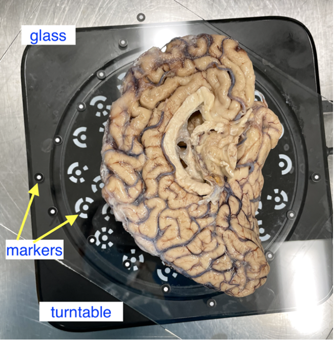
Sample placement on the turntable with sample lateral side down.
Two scan projects are created for all specimens at opposite orientations. For hemispheres, we first acquire a scan with the sample medial side down. Next, the hemisphere is flipped to be lateral side down. Again, to reduce sample movement, we wipe down excess fixative on the sheet of glass to improve traction. Whole Brains are scanned upright (brain stem down) and upside down. Although these types of samples do not tend to move during the scan, they can deform between the two orientations, which can lead to small errors in the final surface reference.
Note: Samples should have the cerebellum removed before acquisition. The cerebellum is not considered in the reconstruction as it is not on the imaged slabs, including it in the scan will lead to incorrect slice reconstruction.
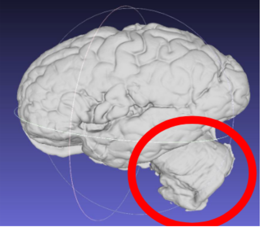
Scan incorrectly including the cerebellum.
Handheld Scanning
Handheld mode can be particularly useful for fresh tissue, since it cannot maintain its shape or be flipped for two-sided scans because of deformation. In this mode, a transparent surface can be used to scan both sides of the sample without having to shift the easily deformable tissue.
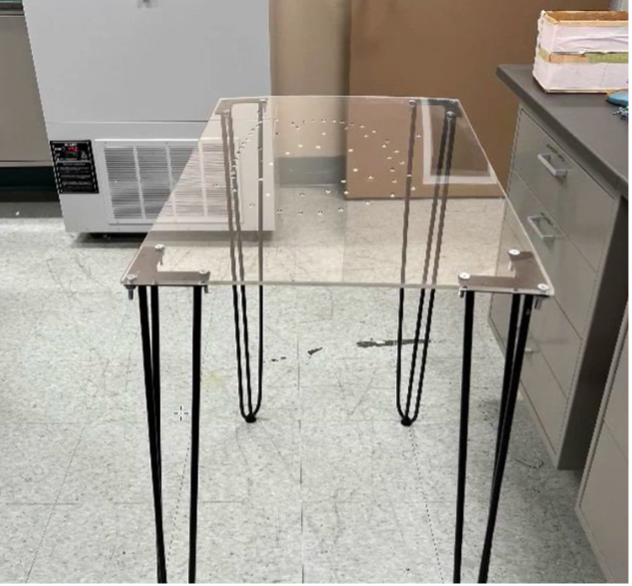
Example of a handheld scan setup.
Running the Scan
In the scan workspace, use the preview window to center the tissue in the center of the field of view. Set the red crosshairs to the middle of the specimen for full coverage as the turntable rotates.
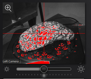
Scanner preview.
The camera exposure has a large effect on scan quality. Incorrect exposure can lead to noisier surfaces in the resulting scan point clouds. Adjust exposure in the main scan menu under the camera preview screen.

Scanner exposure slider.
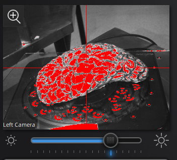
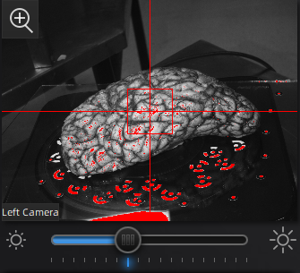
Use the preview window to check exposure, areas that are overexposed will appear red. A good exposure will show some red areas but too many, see below for a reference of a good exposure. For specimens with particularly difficult lighting HDR mode can be used to better render darker features.
|
|
|
||Overexposed (red filter on sample + bright image) ||Underexposed (black filter on sample + dark image) ||Sufficient exposure (can see sample, markers, decent contrast) ||
HDR Mode
HDR mode is used for samples with dark features like bruising or veins. This mode captures three images at each turntable step at different exposures which better capture darker and deeper structures in the tissue (e.g., sometimes this mode is good if point clouds aren’t generated near medial structures, including 3rdventricle, septum pellucidum, corpus callosum, parahippocampal gyrus, occipitotemporal gyrus, and any optic structures – nerve, chiasm)
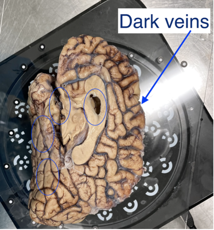
Sample with dark veins.
Editing and Saving Point Clouds
Removing Excess Elements
- Remove excess data or turntable markers using the deleting tool if the scanner picks up other neighboring geometry.
- Select extra elements by holding the shift key and left click.
- Delete these points by clicking the “Delete Selected Data” button or pressing the delete key.
- Press the “Complete Editing” check-mark icon once all necessary edits are done.
- Note: Editing point clouds is easier than editing meshes so make sure to remove any excess elements before generating a mesh.
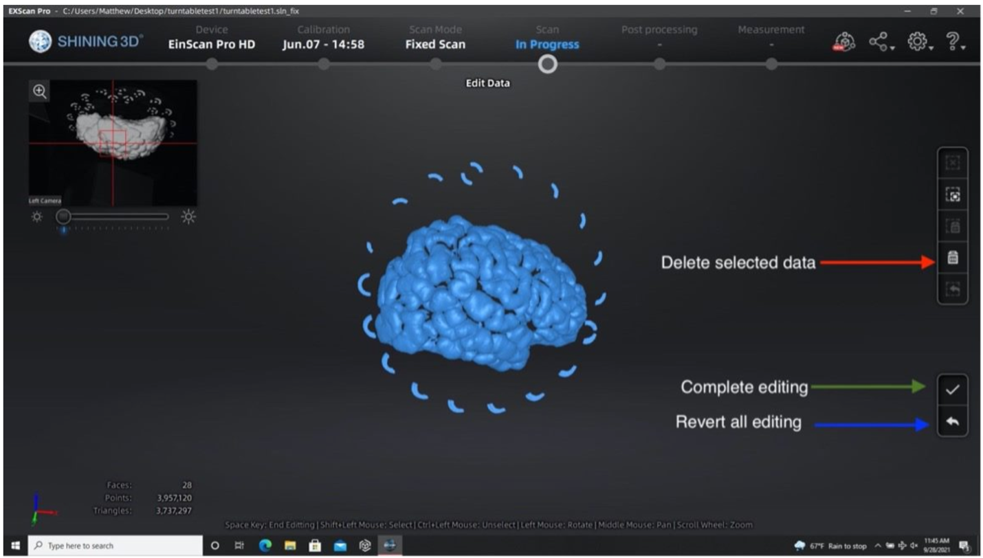
Performing the second run after removing excess elements from the first set of point clouds.
- When finished editing, a point cloud will be generated, which should have saved automatically as “Project 1.”
- Briefly QA scan data, looking at noise or holes in the surface of the scan. Some gaps in the point clouds are normal. Any scan can be redone or added onto to get better results at any time.
Aligning both runs
If you have two scanning sessions, there are a couple of ways the point-clouds can be registered, an automatic and manual method. Only use manual alignment if the automatic method fails.
- Click the alignment icon and select both scanning sessions. Click the automatic alignment button at the top left of the screen. If the alignment fails, continue with the next steps.
- Hold the shift key and left click to select three collinear points on each scan session. Ideally, we would want to place one point on the anterior, superior, and posterior sides of the brain. Spread out points as much as possible to get the best alignment.
- Click Complete when finished with the alignment.
Creating a Mesh
- Click on the global optimization and confirm the resulting point cloud.
- Click on the mesh icon to generate a mesh model from your generated point clouds.
- Select watertight, which will create a mesh that is closed and has no holes.
- Choose the “high-detail” option for the best mesh resolution.
- Select "No filter" so no smoothing is applied on the mesh.
- This reconstruction should take approximately 3+ minutes, depending on the equipment.
- Save your mesh when reconstruction has finished. Your mesh should be saved as a .stl file automatically, but it is also recommended to save your point clouds (.asc files).
Addressing mesh quality
When acquiring the mesh, the sides of the sample are critical for proper point cloud alignment. Poorly captured sides will lead to inaccurate alignments between scans, which will cause issues in the final reconstruction. The following example shows a handheld scan where the sides of the tissue were not acquired, resulting in a flatter/thinner appearance which will negatively affect the quality of the final reconstruction.
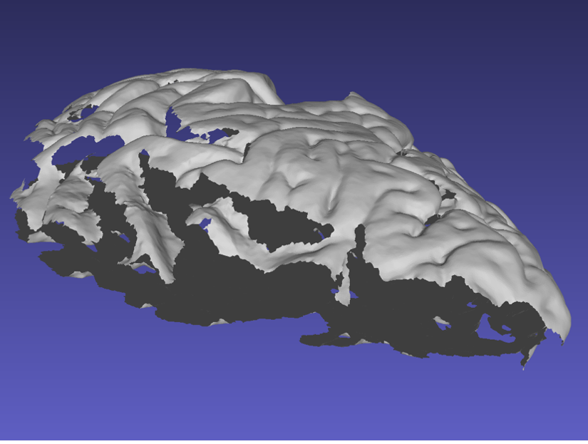
Mesh missing sides of the top scan.
Ideally, the sides of the mesh should be captured as shown in the following example. When performing a handheld scan, it can be difficult to acquire the sides of the sample without acquiring other surfaces. These additional surfaces can be edited and deleted in the same way markers are removed.
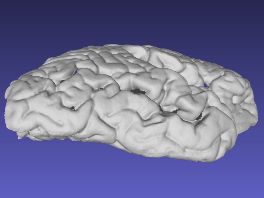
Mesh correctly including the sides of the tissue.
Note that the previous surface has some holes due to deep sulci, which should not pose a problem with the reconstruction. Watertight meshing should be able to handle small gaps in the point-cloud.
Preparing Slab Data
The following guidelines should be followed when preparing slab images for optimal results.
Guidelines for Brain Slab Image Acquisition
There are some important requirements for the photographic setup of the brain slabs to ensure the best results.
Use a high-contrast background that stands out in uniform contrast to the brain slabs, such as a solid black background. This will make slabs are easier to segment downstream. Using a complex background with color similar to your brain slabs, will lead to a more manual intervention such as having to manually trace contours, which is not only time-consuming but also non-reproducible.
|
|
Difficult to segment low contrast background. |
Easy to segment high contrast background. |
Additionally, all tissue block faces must be facing the same direction. All slices should be either from an anterior or a posterior view. Note if slabs are from the posterior view, an extra flag,
--photos_of_posterior_side must be used for the final reconstruction.
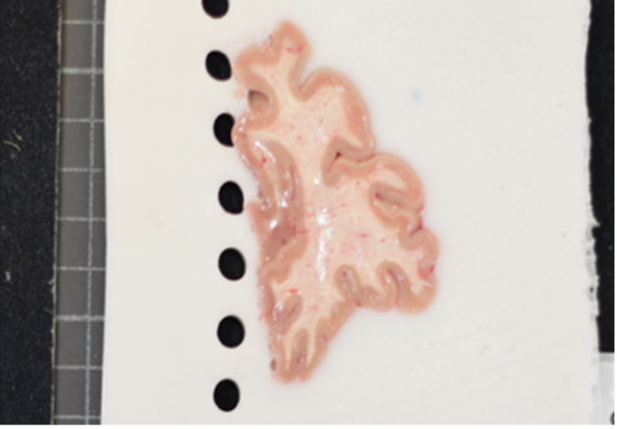
When a single slice produces multiple tissue blocks, they should be placed as similar to the original anatomy as possible. For example, after acquiring slices from the frontal pole, the initial blocks corresponding to the temporal lobe will often be detached from the main block. The following figure shows a) Proper anatomical placement of tissue and, b) Tissue placed too far apart, which is not anatomically accurate.
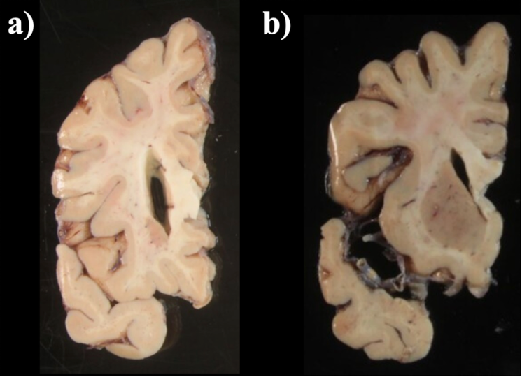
Tissue slab placement a) Properly placed tissue b) Tissue placed in a non-anatomical manner.
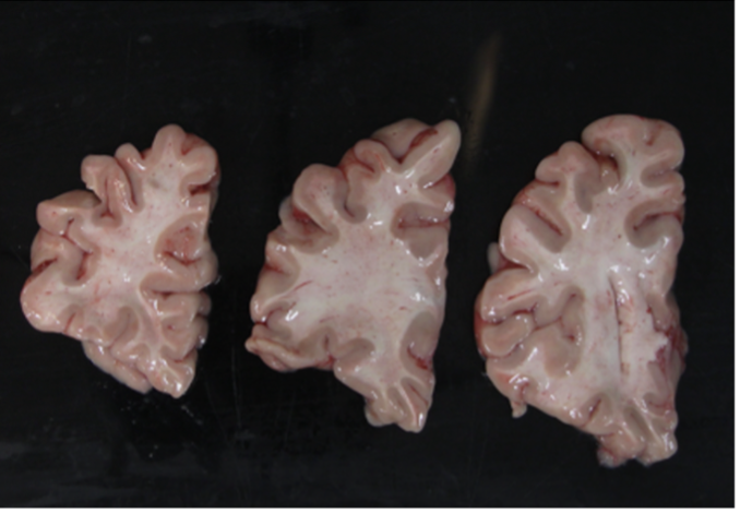
Another example of difficult tissue placement can be the corpus callosum. In the following figure, we see a good example setup with high contrast for the background and good lighting. However, the placement of the corpus callosum on the rightmost slab is incorrect, which will negatively affect volumetric estimates of the third ventricle.
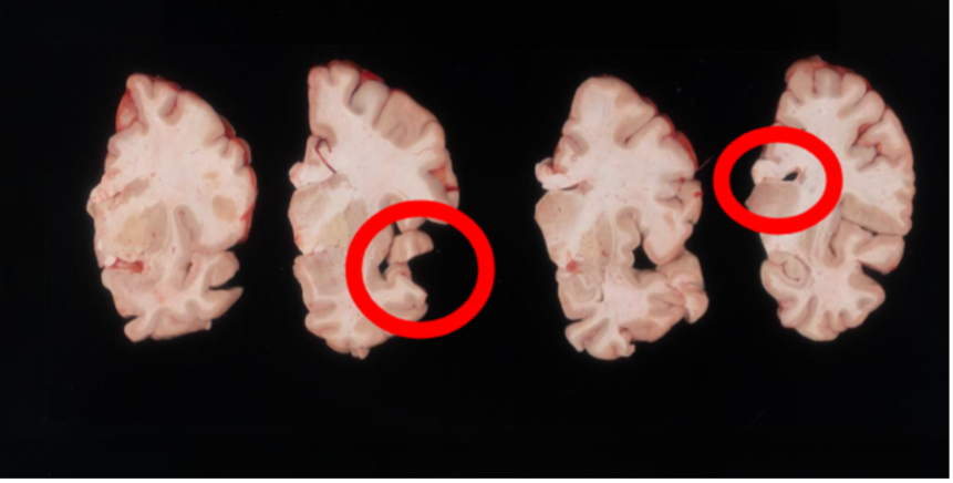
Markers for pixel and perspective corrections
To calibrate pixel size, we will need landmarks with known distances in between them to be provided by the user. The minimum requirement is a ruler, which provides us with two discrete landmarks. This enables rough This method is preferable for legacy images that only have a ruler for reference.
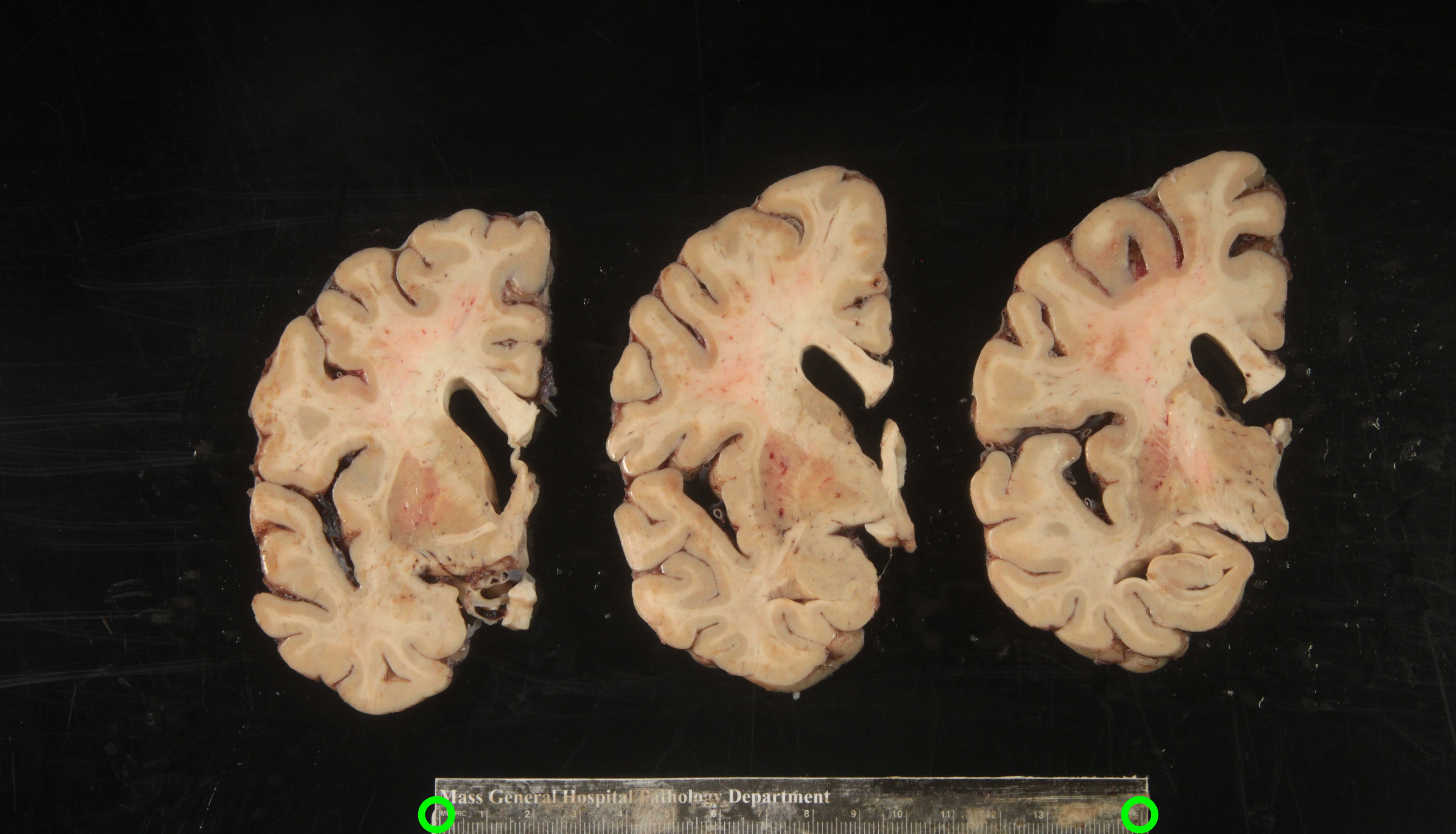
Tip: It is better to use landmarks that are as far apart as possible, as the relative error when manually setting the reference in pixels per millimeter decreases with greater distances.
A more effective setup involves four landmarks placed the corners of a rectangle of known dimensions. This enables us to correct for both pixel size and perspective. In the example below, we can easily tell that the 4 points marked on the grid define a rectangle of dimensions 170x200 mm.
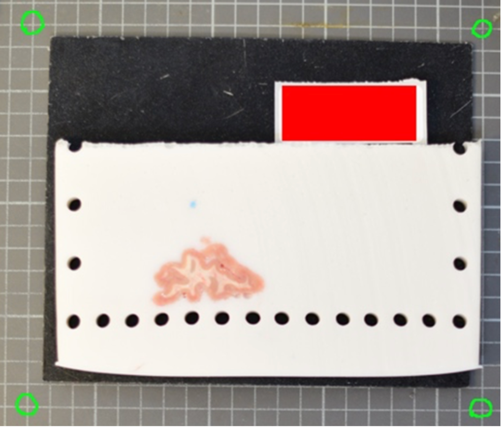
The optimal scenario is to have 4 points defined by fiducial markers with highly salient features. This enables our software to automatically recognize the fiducials, which minimizes human interaction, reducing time and maximizing reproducibility. We strongly recommend that you print these set fiducials and place them on the corners of the board.
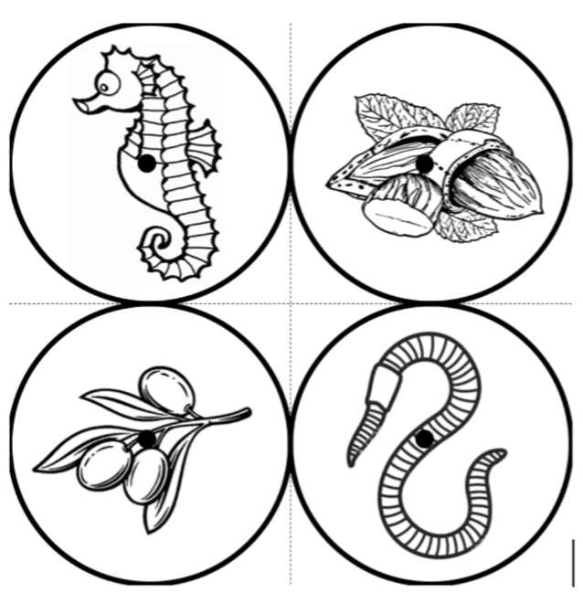
Tip: For best results, affix these fiducials to a small piece of rubber/wood/plastic that lifts them X mm above the board, where X is the thickness of your typical brain slice. Lifting the fiducial minimizes error due to the surface of the brain slice not being at the same distance as the plane of the board surface, but rather a few millimeters above it.
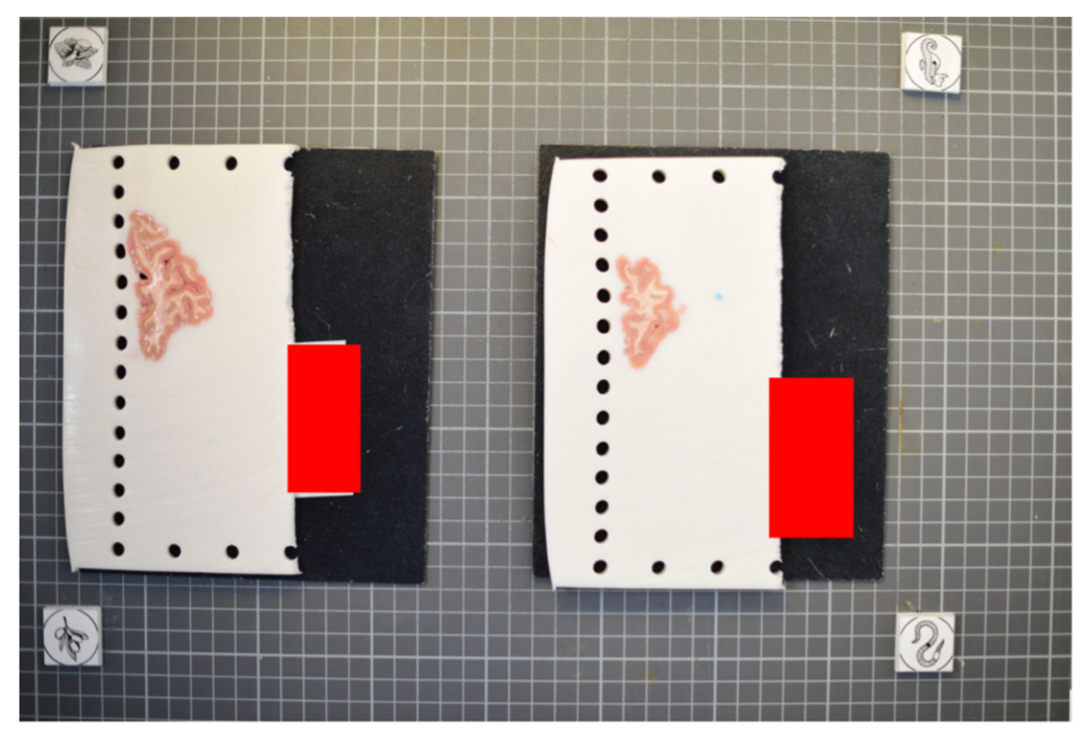
The fiducial form the four corners of our corrected image; hence all tissue should be within the rectangle created from the four fiducial corners. The following image shows slab photos where the fiducials were not placed sufficiently apart.
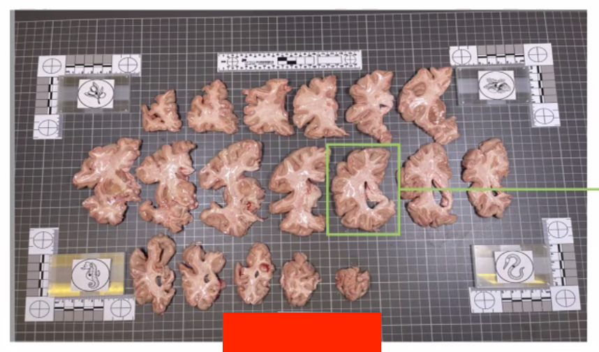
By drawing a rectangle with all fiducial markers, it is clear that much of the tissue lies outside of the pixel-corrected region.
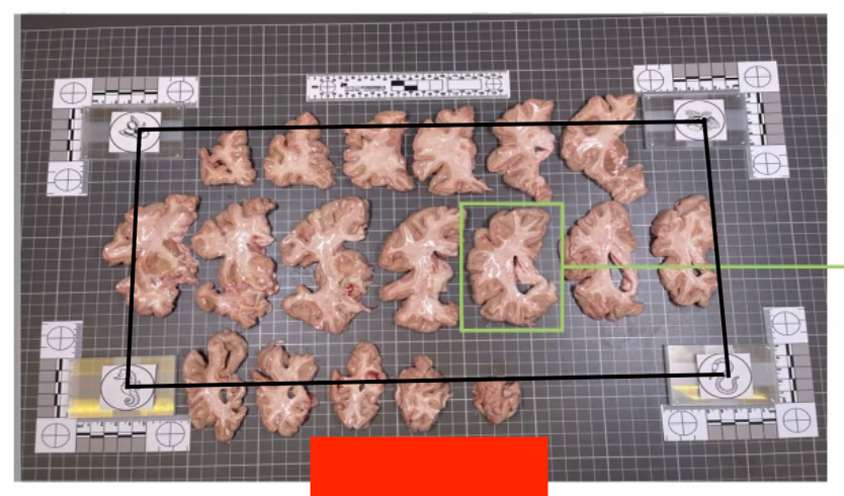
In summary, here is an example of what an optimal photographic setup would look like, including the uniform, high-contrast background and provided fiducials located at known distances, and consistent lighting on all slabs.
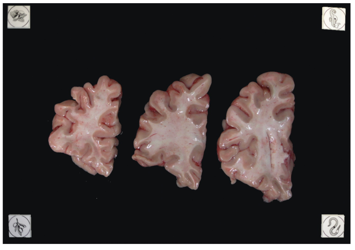
Tip: It does not matter if slabs are not presented on a grid, as long as the distance between the fiducials is known. The software will draw digital rulers for your images later pixel-correction.
Software Installation
The following guide will walk through the steps to install the necessary software for processing the brain slab images and creating the final reconstruction.
Installing Freesurfer
To install Freesurfer, follow the instructions on the Freesurfer website to download the latest stable release, note the tools in this tutorial are scheduled to be released in stable version 7.5: https://surfer.nmr.mgh.harvard.edu/fswiki/DownloadAndInstall
The development version of Freesurfer can be installed by going to this site, where daily updated builds of the software are available: https://surfer.nmr.mgh.harvard.edu/pub/dist/freesurfer/dev/
Alternatively, Freesurfer can be built from source by cloning the Freesurfer repo on github https://github.com/freesurfer/freesurfer and following this guide: https://surfer.nmr.mgh.harvard.edu/fswiki/DownloadAndInstall
Downloading Segmentation Model Weights
The photo reconstruction pipeline uses a nnUNet neural network model to segment the brain slabs to decrease the time involved in manually segmenting photographs. When running dissection_photo_gui you must point to the directory where the model weights are stored. The model weights can be downloaded from the following link:
https://ftp.nmr.mgh.harvard.edu/pub/dist/lcnpublic/dist/dissection_photo_model/nnUNetTrainer__nnUNetPlans__2d.tar.gz
After downloading, extract the files to a directory of your choice. It is recommended to store them in the following Freesurfer directory, as it will be the default location our GUI uses. $FREESURFER_HOME_FSPYTHON/models/
Recommended Directory Structure
We recommend the following directory structure for data and case organization. Each case should have its own directory, and within each case directory, create the following seven subdirectories to store the respective outputs:
- photos – Brain slab images (.JPG, .PNG).
- deformed - Pixel-corrected images.
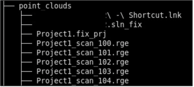
- point_clouds – Files from the project collected from the surface scanner.
- mesh – Watertight mesh processed from point clouds on the scanner (.stl).
- masked – Binarized masks created from pixel-corrected photos.
- connected_components - .npz files showing the connected components for each image.
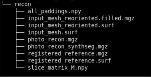
- recon - Final reconstructed volumes, and segmentations.
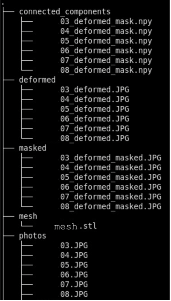
Note that during the image preprocessing GUI files under deformed, masked, and connected_components will be automatically generated. After each step, ensure that your data is saved to the appropriate subdirectory. Below is an example of how files should be organized in the recommended structure:
|
|
Photo Preprocessing
The following guide will walk through the steps to preprocessing the brain slab images. This includes pixel correction, binarizing images, and selecting connected components. Make sure Freesurfer is properly sourced, and you have downloaded the model weights before continuing with the tutorial.
Pixel Correction Using Fiducials
Using the provided fiducial markers, we can correct for non-uniformities in pixel size across the images. If not available this step can be skipped retrospective correction modes can be used in the dissection_photo_gui covered in the next section. For images with fiducials, a calibration is required for pixel correction. For best results, use an image of the setup without tissue.
To start the fiducial calibration use command fiducials_calibration
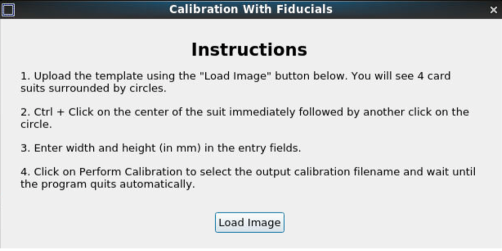
After loading the image, start the calibration process.
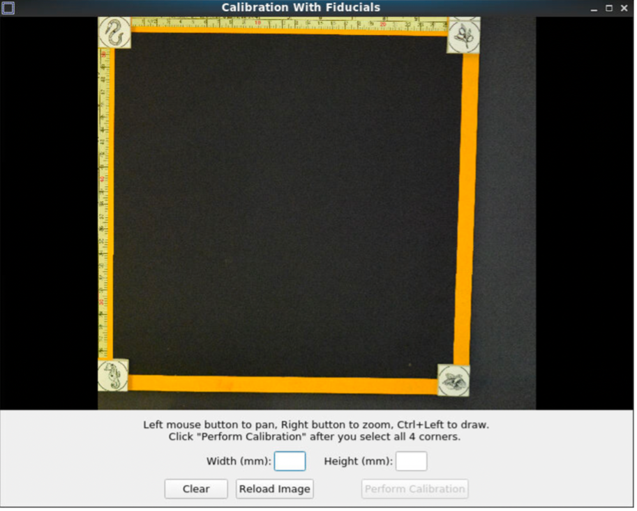
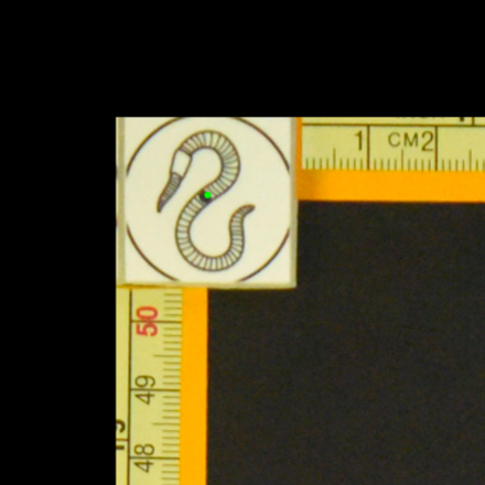
Pan and zoom can be used to have a precise selection in these GUIs. First, select the center of one of the fiducials, followed by selecting the outer ring.
|
|
The first selection at the fiducial center. |
The second selection at the outer circle of the fiducial. |
After selecting all the points, set the width and height between the fiducial markers. Next, click “Perform calibration,” to save a calibration '.npz' file. This calibration file will be used for automating pixel correction in subsequent steps, as long as the fiducial markers are not moved.
Dissection Photo GUI
The dissection photo GUI performs all preprocessing tasks, including pixel correction, binarizing images, and selecting connected components. Before running the GUI, ensure these two environment variables are set if additional files are not in the default locations.
NNUNET_SCRIPT_DIR: This will point at the directory where the file "process_directory_no_upsample.py" which is used to preprocess images before running nnUNet. By default this will point to $FREESURFER_HOME_FSPYTHON/python/packages/nnUNet_v2 but can be changed if images are to be preprocessed differently.
NNUNET_MODEL_DIR: This variable should point to the directory where the nnUNet model weights were downloaded in previous steps are stored. By default this will point to $FREESURFER_HOME_FSPYTHON/models/nnUNetTrainer__nnUNetPlans__2d This can be changed if the models are stored elsewhere.
To run the GUI, source Freesurfer and use command dissection_photo_gui.
Pixel Correction
In the first menu of the dissection_photo_gui select the input directory with the unprocessed gross photographs. Photographs should be set in the order such that tissue slabs are seen in the order they were cut. Additionally select the output directory where the pixel-corrected images will be saved. Here we have the option to load an optimal calibration file if available to automate pixel correction. Select Go! when you have defined the required directories.
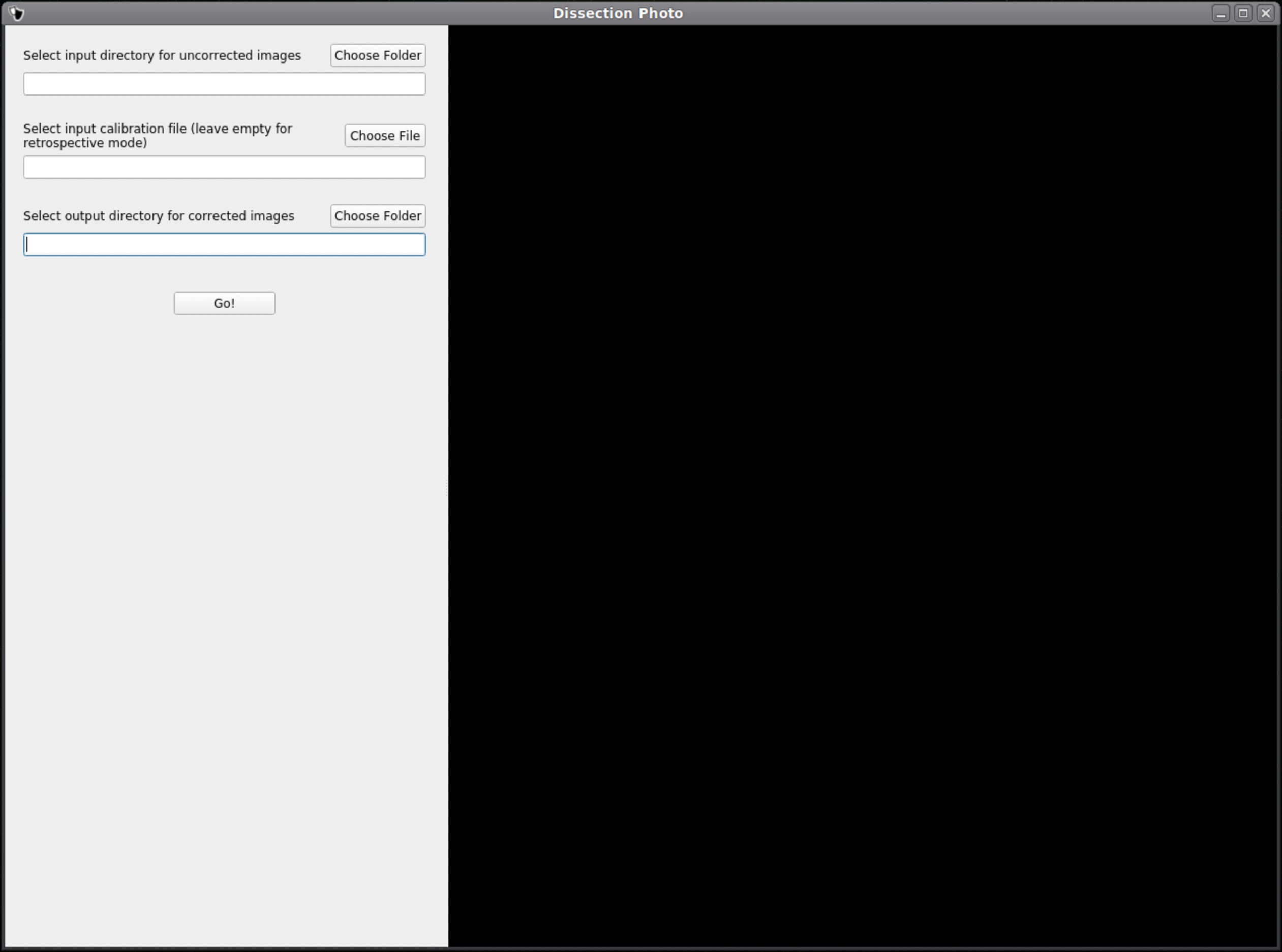
If a calibration file was used the next widow will display the pixel-corrected images for quality assurance purposes. Click Next to proceed assuring the images were corrected.
If no calibration file is provided the next window will be for the Retrospective Correction mode. Select the type of calibration, 2-point, 3-point, or 4-point, and its relevant dimensions in millimeters. The 2-point calibration is used when there is a single axis of ground truth measurement (i.e., One ruler in the image), and four should be chosen if there are two axes, as it will also correct for perspective. We can pan and zoom to make precise selection on the image.
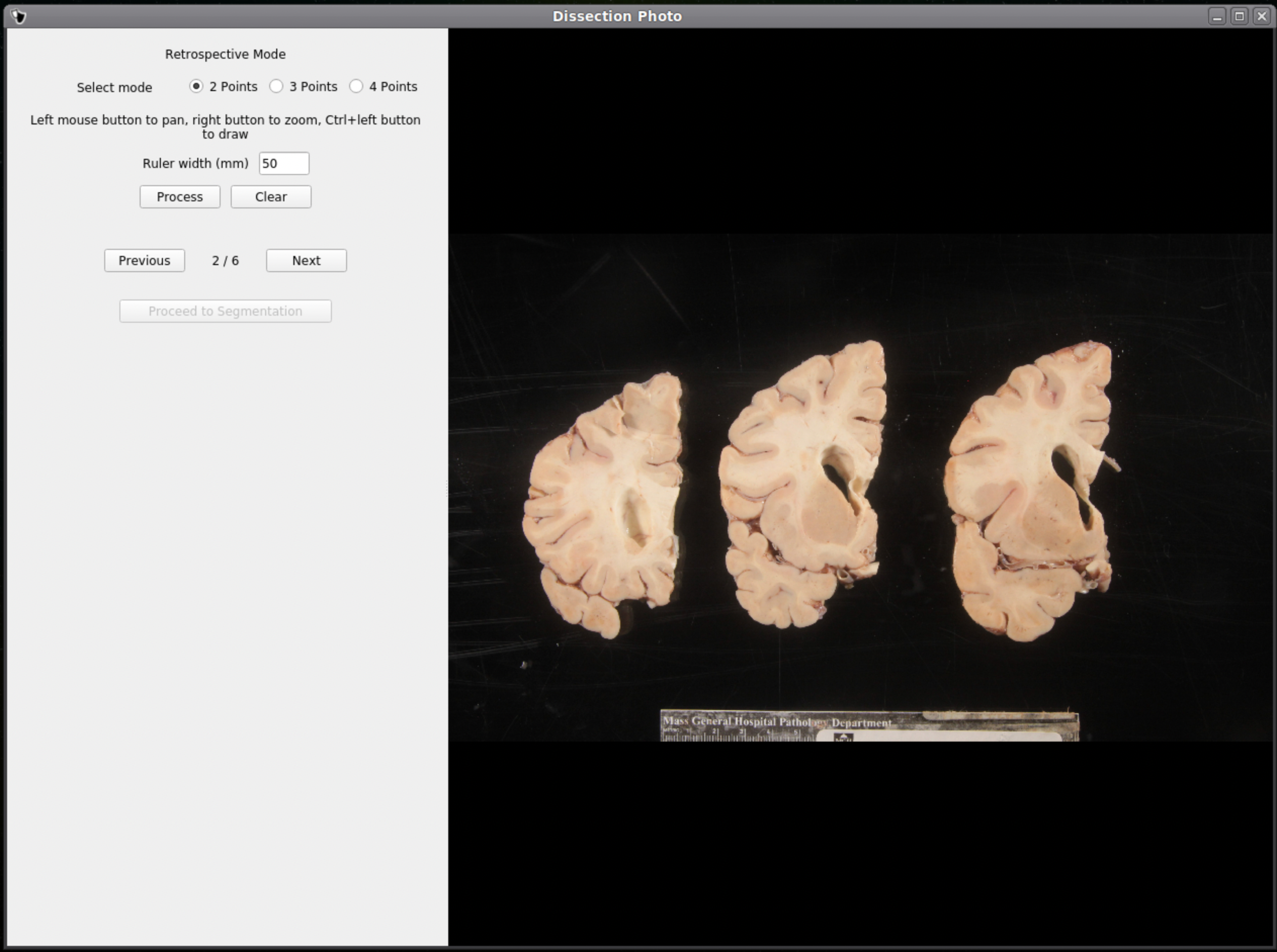
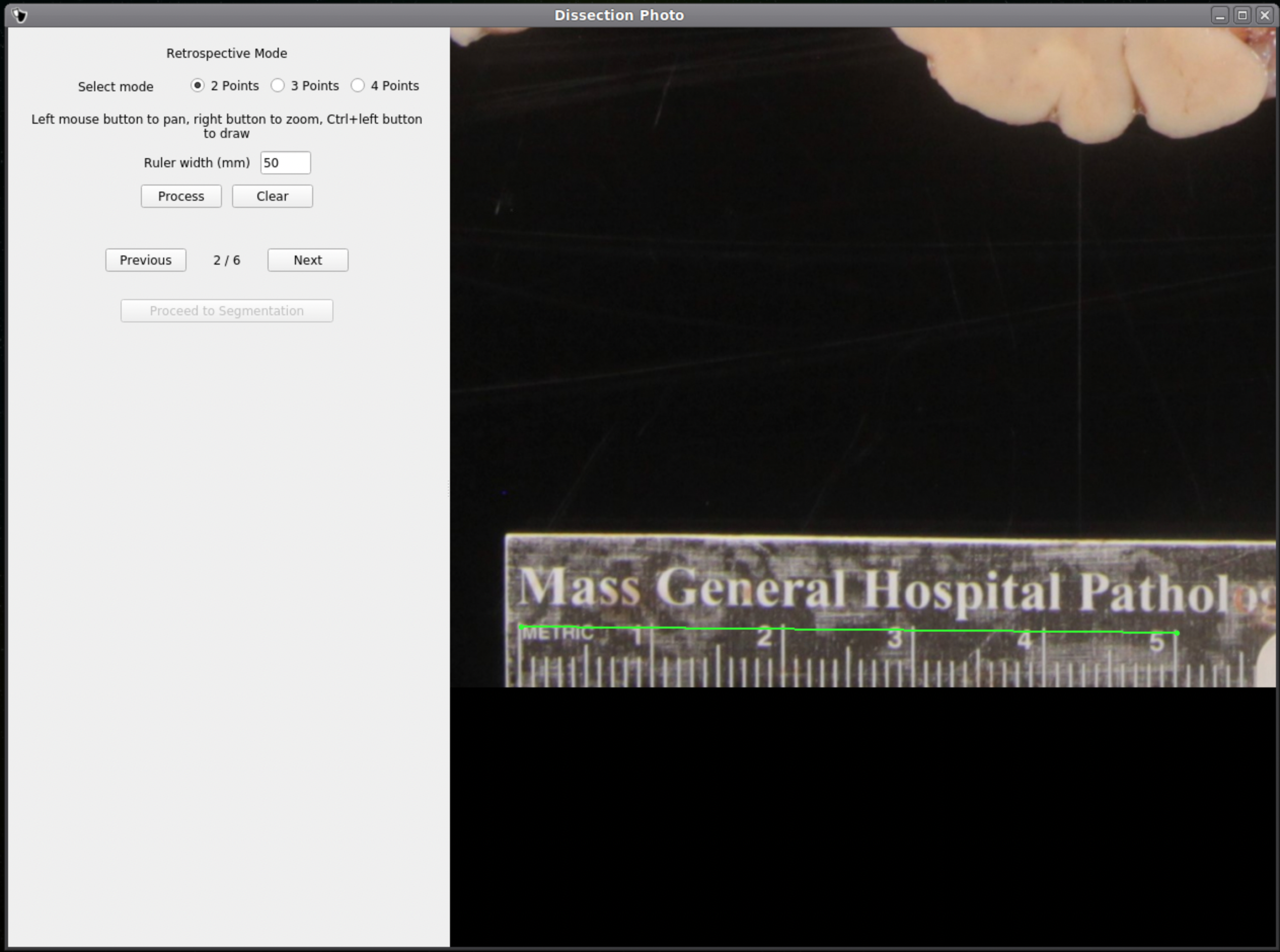
After pixel correcting all images, click Proceed to Segmentation to continue to the next step.
Tissue Segmentation
After selecting an output directory for the masked images, our automatic segmentation tool will immediately start predicting a binary mask per each photograph. If a GPU is available all five folds of the model will be run which will slightly increase segmentation accuracy. After the first photograph is segmented by the model, the user can start cleaning the predicted binary masks. Here the user can pan and zoom like before, but can additionally use a brush tool to remove or add any pixels. Remove any non-slice tissue and the background. The opacity of the predicted mask can also be changed using the provided slider, or toggled using Ctrl+Z.
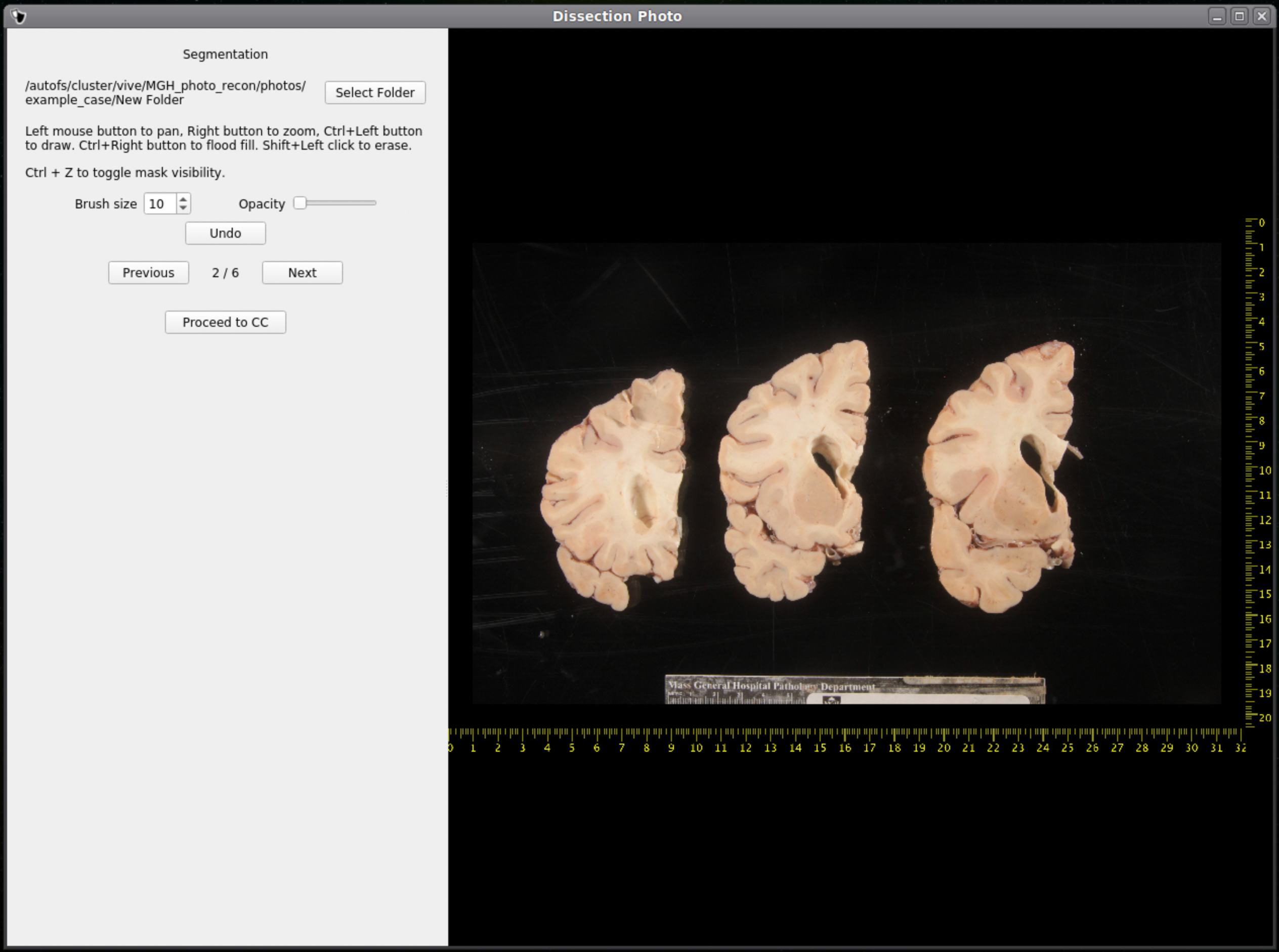
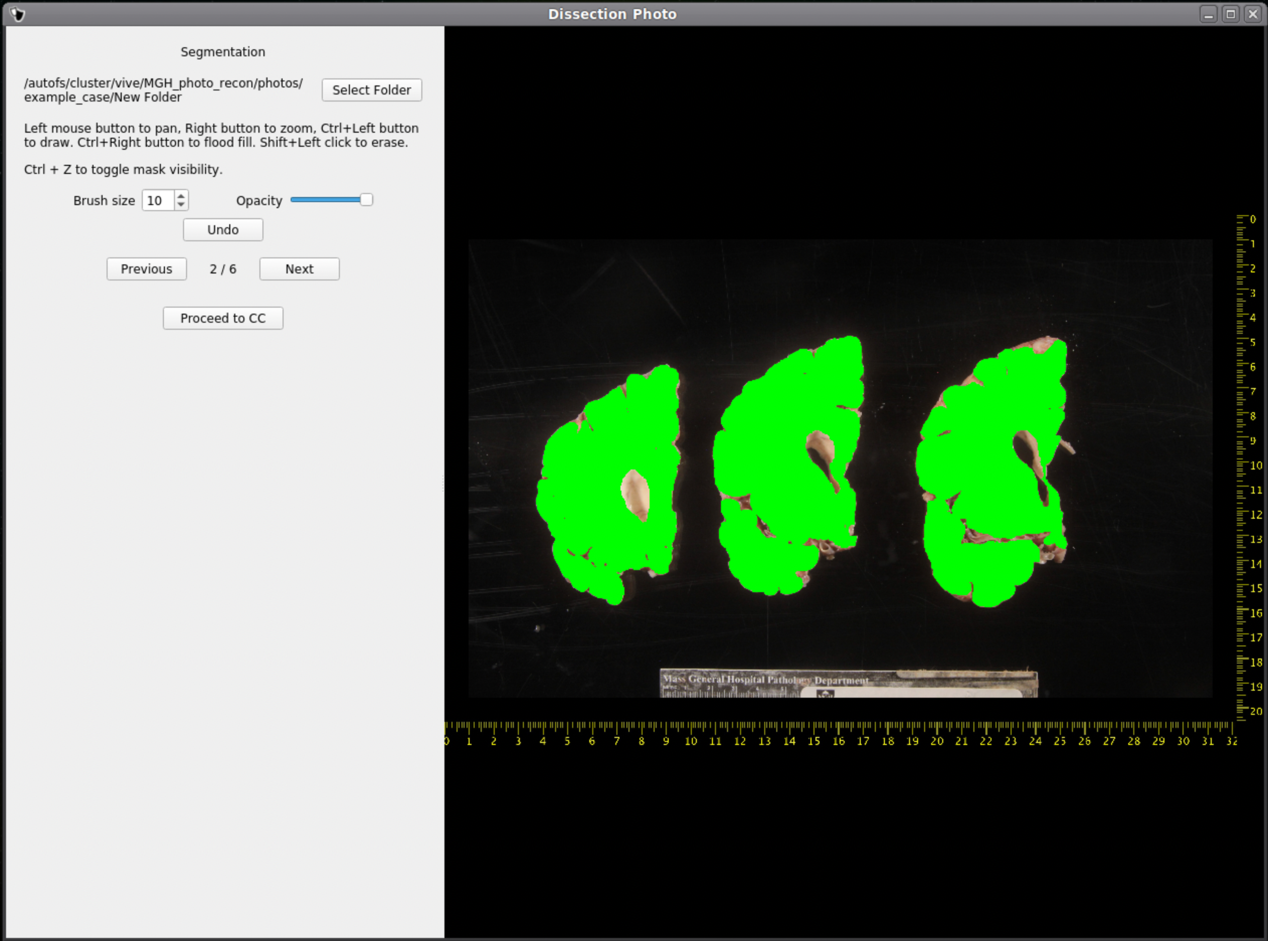
IMPORTANT: The cortical surface should not be part of the masks, so the first (if photographed from the anterior side) or last slice (if photographed from the posterior side) should NOT be considered. You can either leave it out of the mask or ignore it when processing with the GUI.
Once we are satisfied with the mask, click Next to proceed to the next image. After all images have been segmented and cleaned, click Proceed to CC to continue to the connected components step.
Connected Components
Like previous steps, select an output directory for the connected components masks. The connected components section of the GUI will display the masked and pixel-corrected photographs. Here the user will draw boxes around the tissue slabs in each photograph. The GUI will then save the connected components as .npy files.
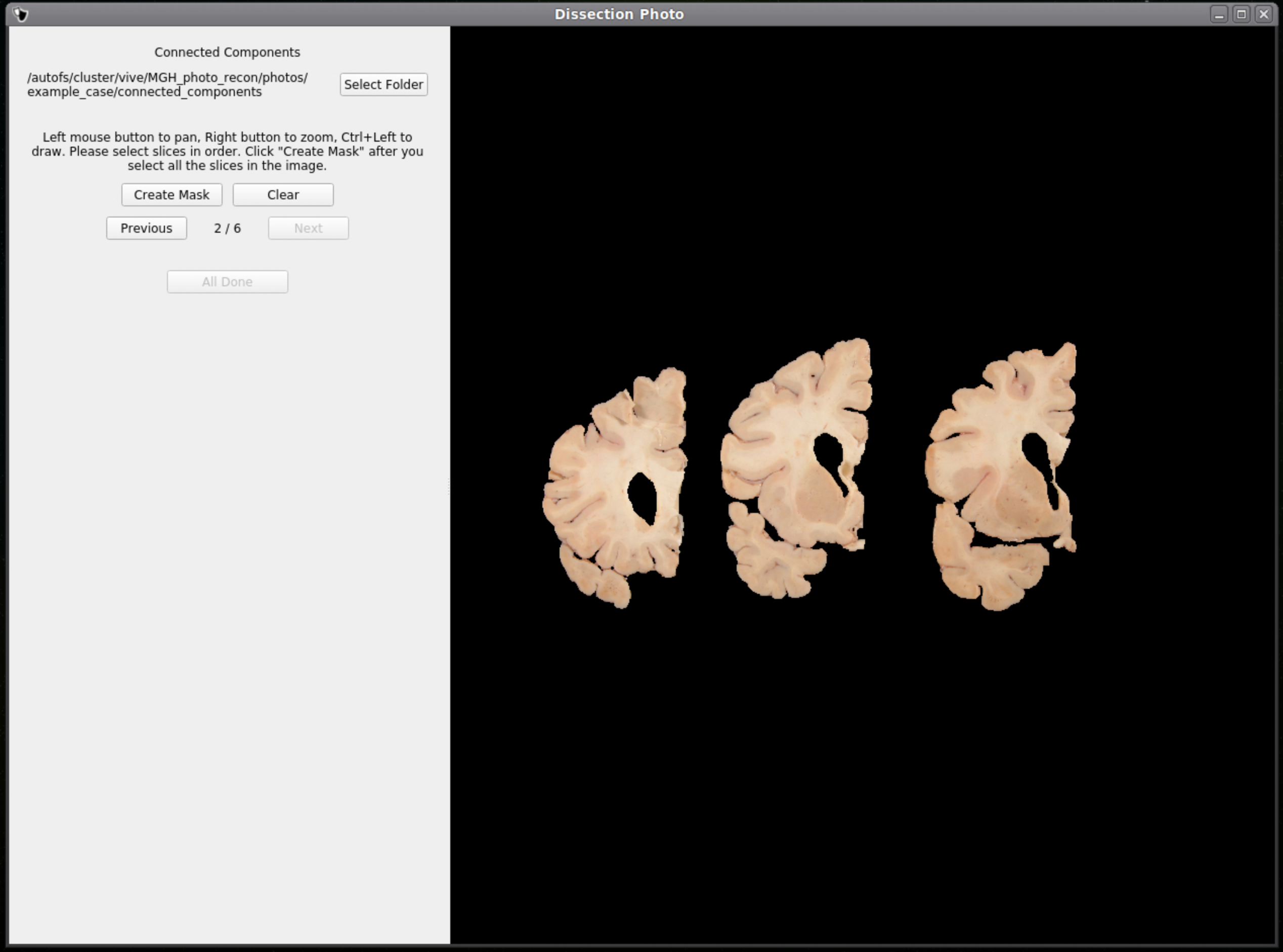
For each image select slices in order, either anterior-posterior or posterior-anterior. Remain consistent of slice order on all photographs. Connected components are selected by clicking and dragging to draw a box in a region of each individual slab in the photograph. After a box has been drawn in each individual slab, click Next to save the output .npy file and move to the next image.
Tip: Make sure no boxes are overlapping.
Once a box is drawn over the tissue, the slab will be colored to show what is being included as one slice.
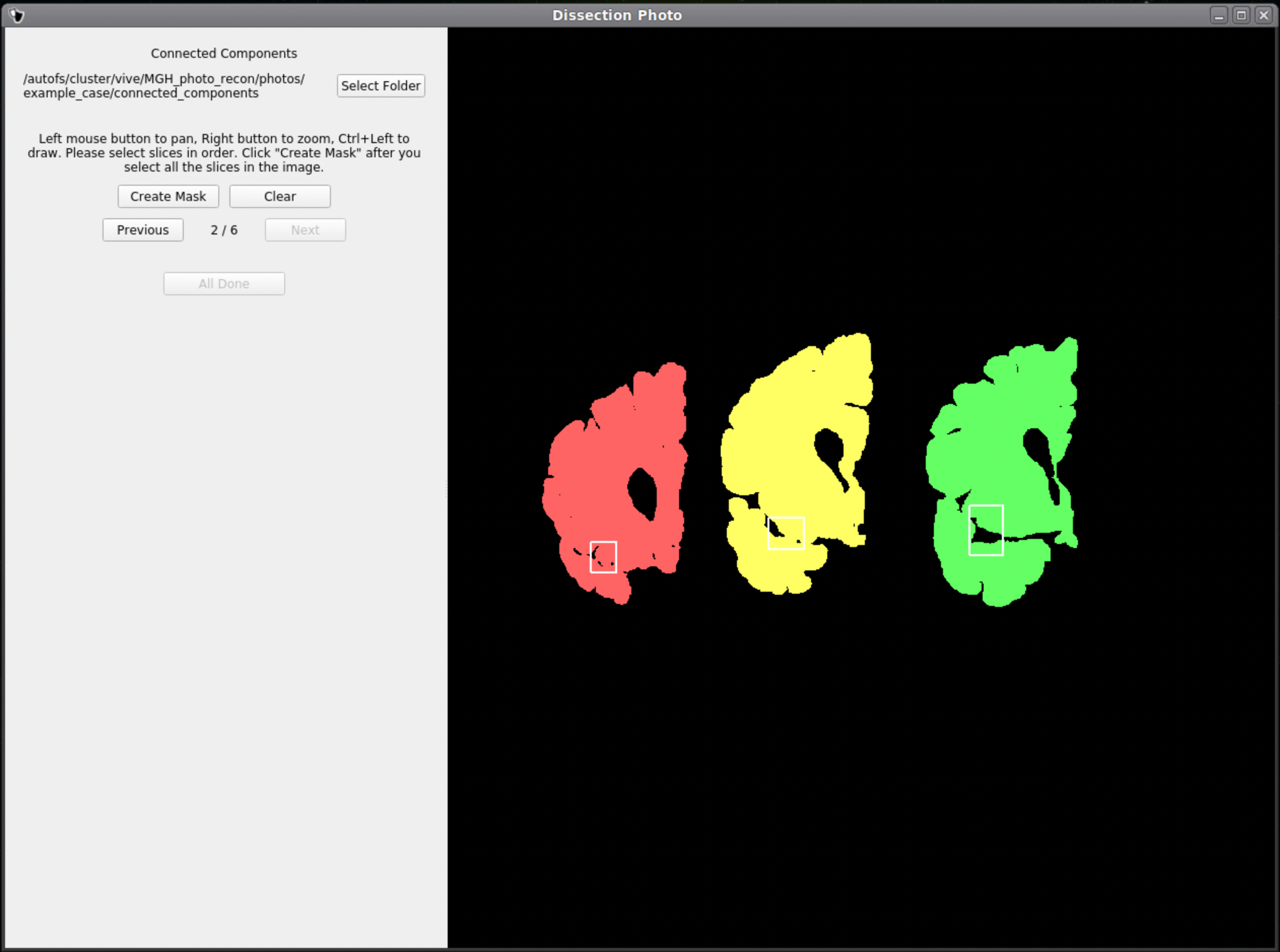
Above is an example of how to correctly draw the boxes within the brain slabs themselves. These boxes inform the GUI that the pixels connected to these slabs are all part of the same tissue slice. Note the box covers tissue from the temporal lobe as it can sometimes be disjoint from the rest of the slab.
Below is an example of how not to draw boxes for this GUI. Notice the occurrence of overlap between boxes and the inclusion of an abundance of black space. Try to keep the boxes drawn to small regions within the brain slabs themselves as to not include any background pixels.
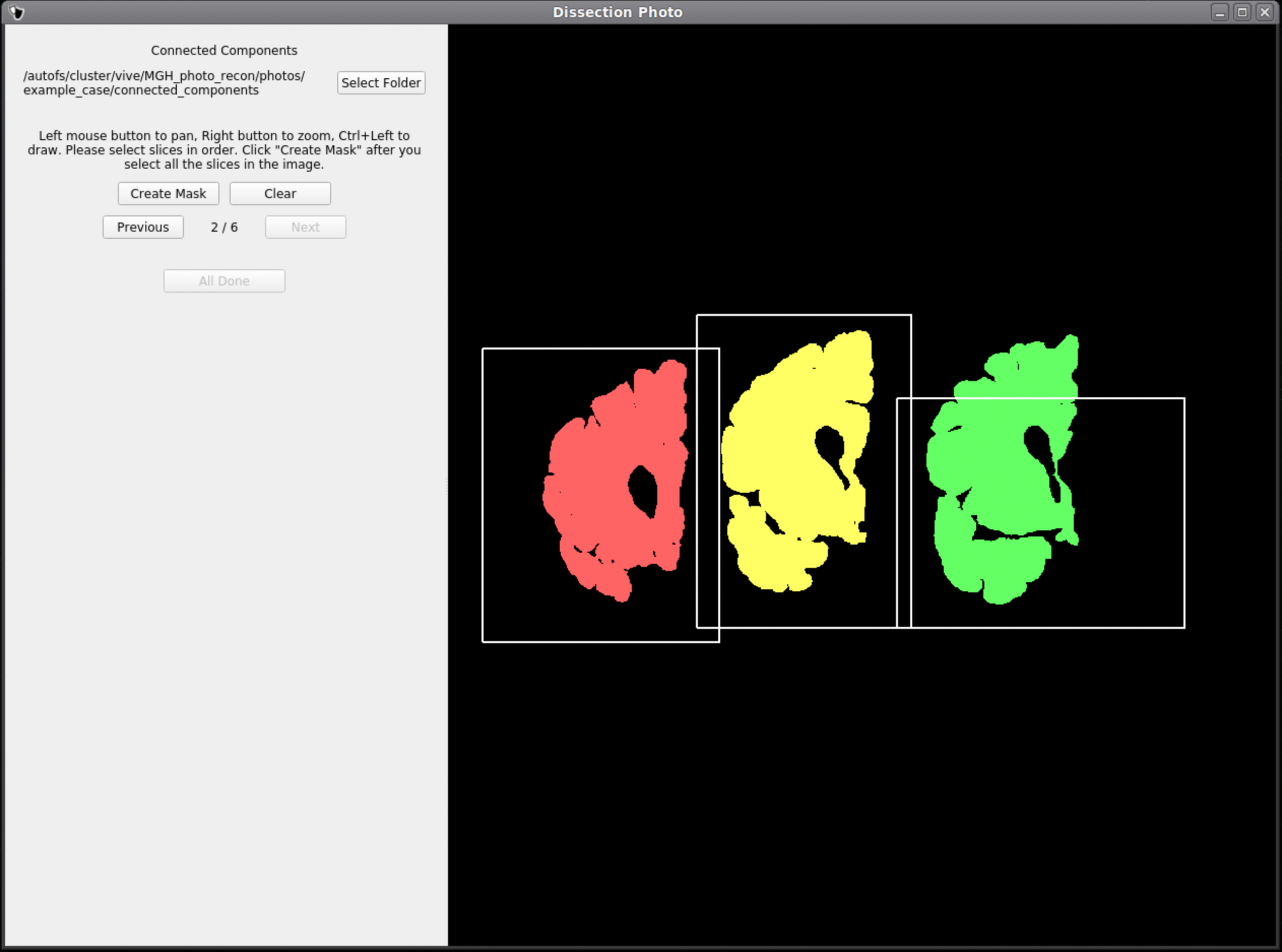
Photo Reconstruction
This is a guide to submitting the final outputs from above aspect to create a 3D reconstruction. Use the following command for help with any flag for the script:
mri_3d_photo_recon -h
--input_photo_dir |
Directory with input pixel-corrected photos. |
--input_segmentation_dir |
Directory with input slab masks/segmentations |
--ref_mask |
When using a binary volume as a reference. |
--ref_surface |
Using a 3D surface scan as a reference. |
--ref_soft_mask |
Using the provided average atlas. Best for using retrospective processing on data without a better reference. |
--mesh_reorient_with_indices |
Vertex indices of the frontal pole, occipital pole, and top of the central sulcus, separated with commas, for mesh alignment. |
--photos_of_posterior_side |
Use when photos are taken of the posterior side of slabs (default is anterior side). |
--order_posterior_to_anterior |
Use when photos are ordered from posterior to anterior (default is anterior to posterior). |
--allow_z_stretch |
Use to adjust the slice thickness to best match the reference. You should probably *never* use this with soft references (ref_soft_mask). |
--rigid_only_for_photos |
Switch on if you want photos to deform only rigidly (not affine). |
--slice_thickness |
Slice thickness in mm. |
--photo_resolution |
Resolution of the photos in mm. |
||--output_directory ||Output directory with reconstructed photo volume and reference ||
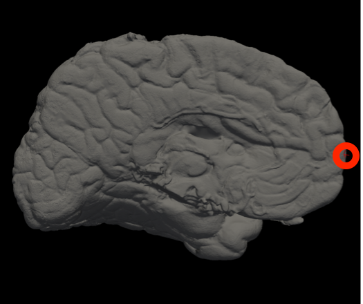
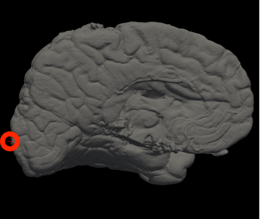
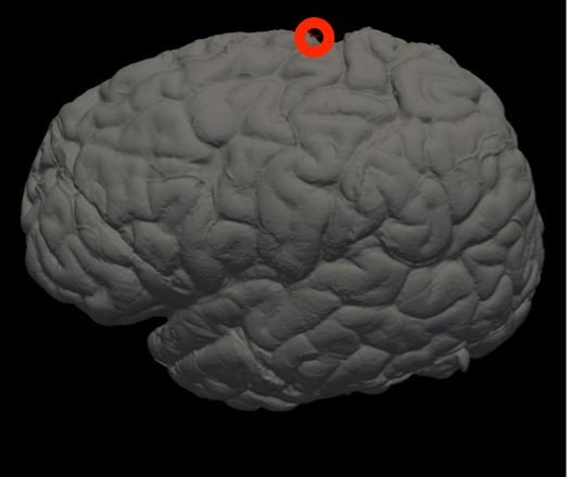
In Freeview, you can find the number corresponding to the vertices of each anatomical area to use in the --mesh_reorient_with_indices flag. These indices should be comma-separated in the order: frontal pole, occipital pole, and top of the central sulcus.
|
|
|
Frontal Pole |
Occipital Pole |
Top of the central sulcus |
For example, the --mesh_reorient_with_indices flag might look like this:
- –mesh_reorient_with_indices 999999,999999,999999
Example for running reconstruction
- mri_3d_photo_recon \
- --input_photo_dir ./deformed \
- --input_segmentation_dir ./connected_components \
- --ref_surface ./mesh/case.stl \
- --mesh_reorient_with_indices 999,1010,333333 \
- --photos_of_posterior_side --allow_z_stretch \
- --slice_thickness 8 \
- --photo_resolution 0.1
Photo-Synthseg Segmentation
The 3D reconstructed stacks can be segmented with SynthSeg using the flag --photo. Please see the wiki page for SynthSeg for further information.
Example for running SynthSeg on a Left Hemisphere
- mri_synthseg \
- --i ./recon/photo_recon.mgz \
- --o ./recon/photo_recon_synthseg.mgz \
- --photo left \
- --parc

