• DraftChallenges

Contour

Introduction to FreeSurfer Output DRAFT

Introduction to FreeSurfer Output

Exercise 1

Difficulty: Beginner

Goal: Practice basic Freeview tasks.

In the examples above you looked at data from a subject called “good_output”. For this challenge complete the following tasks for subject “004”.

1. Open the subject’s aparc+aseg.mgz volume with a colormap of “lut”.
2. Swap the view to sagittal
3. Navigate with the arrow keys to find the right putamen

Need a hint?

• Here is how you opened up a similar volume for the “good_output” subject:  freeview -v good_output/mri/aseg.mgz:colormap=lut 

• Please note that we were in the $TUTORIAL_DATA/buckner_data/tutorial_subjs directory when we used that command - so  cd  there if you'd like to base your command off the above example.

Want to know the answer? Click and drag to highlight and reveal the text below.

Exercise 2

Difficulty: Beginner

Goal: Practice visualizing data with overlays.

1. Open 004’s lh.pial surface, with the overlay named lh.thickness, set the overlay to display with a threshold of 1,2
2. Look up vertex 141813
3. What is the thickness and label of this vertex?

Need a hint?

• Here is how you opened up a similar surface for the good_output subject, with thickness information:  freeview -f good_output/surf/lh.inflated:overlay=lh.thickness:overlay_threshold=0.1,3 --viewport 3d 

• And here is how you opened up a similar surface for the good_output subject with the Desikan-Killany parcellation:  freeview -f  good_output/surf/lh.pial:annot=aparc.annot 

• Please note that we were in the $TUTORIAL_DATA/buckner_data/tutorial_subjs directory when we used that command - so  cd  there if you'd like to base your command off the above example.

Want to know the answer? Click and drag to highlight and reveal the text below.

Exercise 3

Difficulty: Beginner

Goal: Practice opening multiple files at a time with FreeView.

• For this challenge start with this terminal command:

 freeview -v 004/mri/wm.mgz:colormap=jet 004/mri/brainmask.mgz -f 004/surf/lh.pial:edgecolor=blue 004/surf/lh.white:edgecolor=red 

• Right now it only opens the left hemisphere pial and white matter surfaces, alter it to open both for the right hemisphere as well, with colors that match the left hemisphere side.
• Once you have the last command working, rearrange the volume layers in freesurfer so that the wm.mgz is at %20 opacity and the brainmask can be seen underneath it (this can also be done through altering the terminal command - you can choose which way to do so).
• You will need to be in $TUTORIAL_DATA/buckner_data/tutorial_subjs for the command to work, so cd there if needed

Want the solution? Click and drag to highlight and reveal the text below.

Exercise 4

Difficulty: Intermediate - assumes some comfort with navigating Unix and FreeView

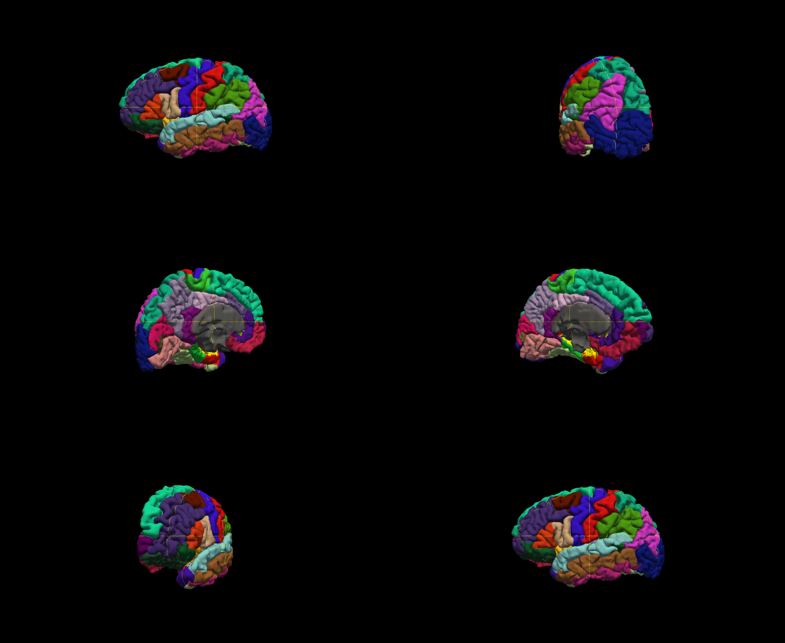
Goal: Export a series of images from FreeView and stitch them together to create a GIF.

1. Open up any surface from the tutorial data

2. Set the viewport to 3d view, right click in the viewport and select  Hide All Slices 

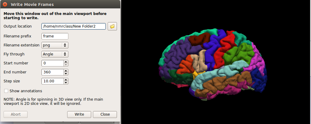
3. In the  File  menu, select  Save Movie Frames 

4. Set up the options as in the following picture - you will likely want to create a new directory in your home directory to save the output to.

5. In a terminal, navigate to the new directory you output the movie data to.

6. Run this command:  convert -delay .1 *.png brainanim.gif 

   • Note: convert is from the ImageMagick library, which is a prerequesite for running FreeView.

   •  -delay  determines the gap between frames,  *.png  selects all png files in the working directory,  brainanim.gif  is the output name.

7. To view your GIF, open it with firefox  firefox brainanim.gif 

Practice Working With Data

Exercise 1

Difficulty: Beginner

Goal: Prepare a dicom series for the recon-all stream

Your goal is to set up your environment variables and assemble the correct recon-all command to process a dicom series.

To begin navigate to the following directory in your terminal:  $TUTORIAL_DATA/practice_with_dicoms 

Take a look at the directories found there. The  dicoms  directory contains a dicom series, and the  subjects  directory is where your recon-all subject output should go. You will want to use dcmunpack to find the first image of the first T1w_MPR_vNav_4eRMS series, set your SUBJECT_DIR environment variable, then then type out and run your recon-all command (use practice_subject as the subject name). Make sure the command starts without any errors - and if it does cancel the process by pressing ctrl and c on the keyboard (a recon-all can take many hours!).

Check in the  work  directory to ensure a directory with your subject's name was created (practice_subject), if you see the folder you have completed the challenge!

Hints:

• Follow the tutorial example for guidance
• It might be tricky to find the path to the subjects directory if you are new to Unix, you can use this: $TUTORIAL_DATA/practice_with_dicoms/subjects

Want to see the answer? Highlight the lines below

Anatomical ROI Analysis

Exercise 1

Difficulty: Beginner

Goal: To practice collecting different types of measures with asegstats2table

Create a table called mean.practice.table that lists the average mean intensities of all segments for subjects 004 021 and 092.

When done use the following command to open up an excel-like program on your computer and look at the data   soffice --calc mean.practice.table  , note, the command may take some time to run and may report warnings which you can ignore. (If you are not at a FreeSurfer course, you may not have this program, in this case use  gedit mean.practice.table  to open the table. )

Hints:

• If you don't specify which segment numbers you want, the measurements will be collected for all segments.

• If you run  asegstats2table --help  you can get a list of all the ways to configure your table, here is some information from that command which might help:

•  --meas=MEAS  measure: default is volume ( alt: mean, std) 

• For example,  asegstats2table --meas std  would add the standard deviation measurements of each segment to the table.

• You will probably want to run  cd $SUBJECTS_DIR  first so you are in the right directory.

Want the answer? Highlight the black lines below to see!

Exercise 2

Difficulty: Intermediate, will present challenges to Unix beginners (but is totally possible!)

Goal: To practice collecting different types of measures and using different atlases with aparcstats2table

Create a table called rh.aparc.a2009.thickness.table which lists the main thickness in all left hemisphere cortical parcellations for subjects 004 021 and 040.

When done use the following command to open up an excel-like program on your computer and look at the data   soffice --calc lh.aparc.a2009.thickness.table  , note, the command may take some time to run and may report warnings which you can ignore. (If you are not at a FreeSurfer course, you may not have this program, in this case use  gedit mean.practice.table  to open the table. )

Hints:

• If you run  aparcstats2table --help  you can see a list of all the different ways to configure your table, here is some information found through that command that might help:

•  -p PARC, --parc=PARC  parcellation.. default is aparc ( alt aparc.a2009s) 

•   -m MEAS, --measure=MEAS  measure: default is area ( alt volume, thickness, thicknessstd, meancurv, gauscurv, foldind, curvind) 

• You will probably want to run  cd $SUBJECTS_DIR  first so you are in the right directory.

Want the answer? Highlight the black lines below to see!

Surface Based Group Analysis

Exercise 1

Difficulty: Beginner

Goal: To practice setting up an analysis on subject surfaces to test an experimental hypothesis.

In the tutorial you just completed you examined the effect of age on cortical thickness, accounting for the effects of gender. In this challenge you will use the same data set to examine the effect of gender on cortical thickness, accounting for the effects of age.

Your goal is to create a new contrast file and alter the commands you used above to examine this new hypothesis. You will then open the new sig.mgh overlay which will highlight significant differences found.

Please name your new contrast file  challenge-Cor.mtx  Please set your GLM output directory to  glm_challenge 

Hints:

• It will help if you start in this directory  $SUBJECTS_DIR/glm  and run all of your commands from there.

• You will want to use  mkdir glm_challenge  to make the output directory, and be sure to use that directory when you run mri_glmfit

• Follow the tutorial for guidance.
• You will not need to change the FSGD file, as you are using the same groups - you don't need to change the descriptor of the groups.

• You can use the command  touch challenge-Cor.mtx  to create a new contrast, and  gedit challenge-Cor.mtx  to edit it.

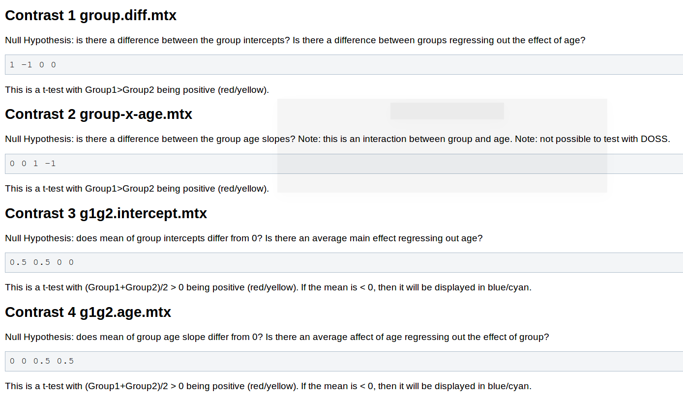
• You will need to adjust your contrasts, consider the following snippet from the wiki page Two Groups (One Factor/Two Levels), One Covariate

• You will not need to pre-process the data, as changing the contrast doesn't have any effect on this stage.
• When you run mri_glmfit you will want to change which contrast it reads and the directory it saves to.

• If you named your contrast  challenge-Cor.mtx  and set your output directory to  glm_challenge than this command should let you examine your significance overlay.

  •  freeview -f $SUBJECTS_DIR/fsaverage/surf/lh.inflated:overlay=glm_challenge/challenge-Cor/sig.mgh:overlay_threshold=4,5 -viewport 3d -layout 1

Want to know the answer? Highlight the text below

Clusterwise Correction For Multiple Comparisons (Permutations)

Exercise 1

Difficulty: Intermediate

Goal: Practice running permutation simulations to correct for multiple comparisons.

Your goal is to run the same permutation operations you learned about in this tutorial on the analysis you created from last tutorial ( where you examined the effect of gender on cortical thickness). In this challenge you will will actually run the permutations (in the tutorial above it was done for you) - but you will do it only run it with 10 rather than the usual 1000 to save time. When done open up the same overlays as you did in the tutorial and see what effect the smoothing did on the analysis.

Hints:

• Follow the tutorial for guidance
• You will want to start working in the directory from last tutorial (because that is where your data is):

 export SUBJECTS_DIR=$TUTORIAL_DATA/buckner_data/tutorial_subjs/group_analysis_tutorial 
 cd $SUBJECTS_DIR/glm 

• You will need to run mri_glmfit again with the --eres-save option, be sure to run it with the contrast and directory you made from before (  challenge-Cor.mtx  and  glm_challenge  )

• When you run the simulation - be sure to change the directory and the permutations count to 10  --perm 10 4.0 abs 

• If you followed the file and directory names specified in the challenge, this command should let you view your output:

  •  freeview -f $SUBJECTS_DIR/fsaverage/surf/lh.inflated:overlay=glm_challenge/challenge-Cor/perm.th40.abs.sig.cluster.mgh:overlay_threshold=2,5:annot=glm_challenge/challenge-Cor/perm.th40.abs.sig.ocn.annot -viewport 3d -layout 1 

Want to know the answer? Highlight below to find out.

Registration

Exercise 1

Difficulty: Intermediate

Goal: Practice using  bb register  to automatically register unaligned data.

Navigate to  $SUBJECTS_DIR/multimodal/fmri/challenge/challenge-template , which contains  template.nii  which is a volume you need to align to a subject named  regsubject .  regsubject  is in the subjects directory that you have already set if you have been following the tutorial above. Name your output for bbregister  register.lta 

You can use the command  freeview -v template.nii $SUBJECTS_DIR/regsubject/mri/orig.mgz:visible=0 -f $SUBJECTS_DIR/regsubject/surf/lh.white $SUBJECTS_DIR/regsubject/surf/rh.white  to inspect the unaligned data first if you would like.

When done, inspect the data to see if it is aligned. Note - the results may be slightly unexpected! If you names your output as requested above the following command should open everything up:

 freeview -v $SUBJECTS_DIR/regsubject/mri/orig.mgz:visible=0 template.nii:reg=register.lta -f $SUBJECTS_DIR/regsubject/surf/lh.white $SUBJECTS_DIR/regsubject/surf/rh.white 

Want the answer? Highlight below to see: