FreeSurfer Analysis Pipeline Overview
Contents
FreeSurfer is a set of software tools for the study of cortical and subcortical anatomy. In the cortical surface stream, the tools construct models of the boundary between white matter and cortical gray matter as well as the pial surface. Once these surfaces are known, an array of anatomical measures becomes possible, including: cortical thickness, surface area, curvature, and surface normal at each point on the cortex. The surfaces can be inflated and/or flattened for improved visualization. The surfaces can also be used to constrain the solutions to inverse optical, EEG and MEG problems. In addition, a cortical surface-based atlas has been defined based on average folding patterns mapped to a sphere. Surfaces from individuals can be aligned with this atlas with a high-dimensional nonlinear registration algorithm. The registration is based on aligning the cortical folding patterns and so directly aligns the anatomy instead of image intensities. The spherical atlas naturally forms a coordinate system in which point-to-point correspondence between subjects can be achieved. This coordinate system can then be used to create group maps (similar to how MNI space is used for volumetric measurements). Most of the FreeSurfer pipeline is automated, which makes it ideal for use on large data sets.
The Surface-based Stream
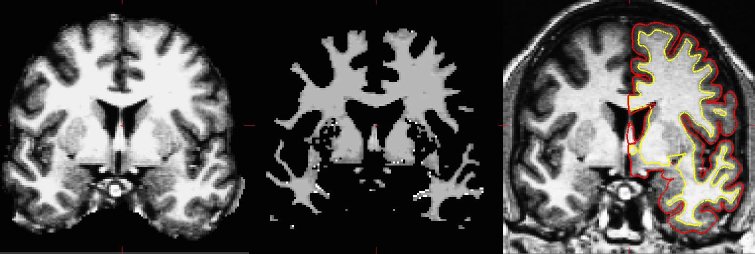
The surface-based pipeline consists of several stages (described in detail in Fischl, et al, 1999a, and Dale, et al, 1999). First, the volume is registered with the MNI305 (Collins et al 1994) atlas (this is an affine registration). This allows FreeSurfer to compute seed points in later stages. The B1 bias field is estimated by measuring the variation in the white matter intensity. The main body of the white matter is used to estimate the field across the entire volume. Likely white matter points are chosen based on their locations in MNI305 space as well as on their intensity and the local neighborhood intensities. The intensity at each voxel is then divided by the estimated bias field at that location in order to remove the effect of the bias field. The skull is stripped (Figure 1A; Segonne, et al, 2004) using a deformable template model. Voxels are then classified as white matter or something other than white matter (Figure 1B) based on intensity and neighbor constraints. Cutting planes are chosen to separate the hemispheres from each other as well as to remove the cerebellum and brain stem. The location of the cutting planes is based on the expected MNI305 location of the corpus callosum and pons, as well as several rules-based algorithms that encode the expected shape of these structures. An initial surface is then generated for each hemisphere by tiling the outside of the white matter mass for that hemisphere. This initial surface is then refined to follow the intensity gradients between the white and gray matter (this is referred to as the white surface). The white surface is then nudged to follow the intensity gradients between the gray matter and CSF (this is the pial surface). The white and pial surfaces overlaid on the original T1-weighed image are shown in Figure 1C. The distance between the white and the pial gives us the thickness at each location of cortex (Fischl and Dale, 2000).

Figure 1: Three stages from the FreeSurfer cortical analysis pipeline. A. skull stripped image. B. white matter segmentation. C. surface between white and gray (yellow line) and between gray and pia (red line) overlaid on the original volume.
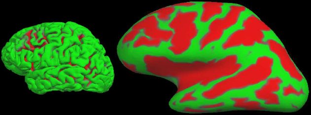
We can also compute the local curvature, surface area, and the surface normal. A 3D view of the pial surface is shown in Figure 3A. This surface can be inflated to show the areas in the sulci as shown in Figure 3B. This surface can then be registered to the spherical atlas based on the folding patterns (Fischl, et al, 1999b).

Figure 3: A. Pial surface. B. Inflated surface. Green indicates a gyrus. Red indicates a sulcus.
The Volume-based (Subcortical) Stream
The volume-based stream is designed to preprocess MRI volumes and label subcortical tissue classes. The stream consists of five stages (fully described in Fischl, et al, 2002, 2004b). The first stage is an affine registration with MNI305 space specifically designed to be insensitive to pathology and to maximize the accuracy of the final segmentation (a different procedure than the one employed by the surface-based stream). This is followed by an initial volumetric labeling. The variation in intensity due to the B1 bias field is corrected (again using a different algorithm than the surface-based stream). Finally, a high dimensional nonlinear volumetric alignment to the MNI305 atlas is performed. After the preprocessing, the volume is labeled (see below). The volume-based stream has evolved somewhat independently from the surface-based stream. The volume-based stream only depends upon the skull stripping to create a mask of the brain in which the labeling is performed. The last stage, actually labeling the volume, is described below.
Label Atlas Construction
Both the cortical (Fischl, et al, 2004b) and the subcortical (Fischl, et al, 2002) labeling use the same basic algorithm. The final segmentation is based on both a subject-independent probabilistic atlas and subject-specific measured values. The atlas is built from a training set, i.e., a set of subjects whose brains (surfaces or volumes) have been labeled by hand. These labels are then mapped into a common space (MNI305 space for volumes and spherical space for surfaces) to achieve point-to-point correspondence for all subjects. Note that a "point" is a voxel in the volume or a vertex on the surface. At each point in space, there exists the label that was assigned to each subject and the measured value (or values) for each subject. Three types of probabilities are then computed at each point. First, the probability that the point belongs to each of the label classes is computed. The second type of probability is computed from the spatial configuration of labels that exist in the training set, which is termed the neighborhood function. The neighborhood function is the probability that a given point belongs to a label given the classification of its neighboring points. The neighborhood function is important because it helps to prevent islands of one structure in another at the structure edges. Third, the probability distribution function (PDF) of the measured value is estimated separately for each label at each point. For volume-based labeling, the measured value is the intensity at that voxel. For surfaced-based labeling, the measured value is the curvature in each of the principal directions at that vertex. The PDF is modeled as a normal distribution, so we only need to estimate the mean and variance for each label at each point in space. If there is more than one measured value (e.g., multi-spectral data), then the PDF is modeled as a multivariate normal for which we need to estimate the mean and variance-covariance matrix for each label.
Labeling a Data Set
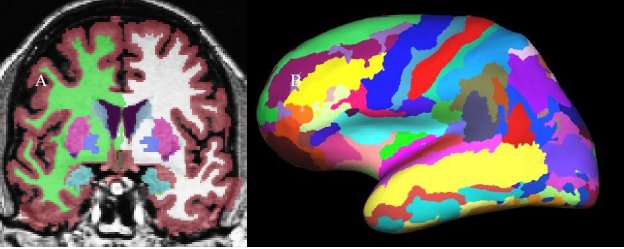
The classification of each point in space to a given label for a given data set is achieved by finding the segmentation that maximizes the probability of input given the prior probabilities from the training set. First, the probability of a class at each point is computed as the probability that the given class appeared at that location in the training set times the likelihood of getting the subject-specific measured value from that class. The latter is computed from the PDF for that label as estimated from the training set. The probability of each class at each point is computed. An initial segmentation is generated by assigning each point to the class for which the probability is greatest. Given this segmentation, the neighborhood function is used to recompute the class probabilities. The data set is resegmented based on this new set of class probabilities. This is repeated until the segmentation does not change. This procedure allows the atlas to be customized for each data set by using the information specific to that data set. Once complete, not only do we have a label for each point in space, but we also have the probability of seeing the measured value at each voxel. The product of this probability over all points in space yields the probability of the input. This will be used later during automatic failure detection. This procedure has been shown to be statistically indistinguishable from manual raters (Fischl, et al, 2002) and relatively insensitive to changes in acquisition parameters (Fischl, et al, 2004a). The results are shown in Figure 4. In 4A, the volumetric labeling shows several subcortical structures (putamen, hypocampus, ventricles, etc). Note that all of the white matter is considered a single label, as is all of the cortical gray matter for each cortical hemisphere.

Figure 4: A. Volume-based labeling. Note that cortical gray matter and white mater are represented by single classes. Also note that there are separate labels for the structures in each hemisphere. B. Surface-based labeling.
Surface-based Statistical Analysis
GLM analysis on the surface enables us to test models of how any surface-based measure might change as a function of demographic or genetic variables, group membership (eg, Alzheimer's disease or normal). This tool will be generalized to allow for FA at a particular point on the cortical surface (or immediately below the subcortical junction) to be used as a parameter in the linear model.
Longitudinal Processing Stream
A longitudinal processing stream is also available in Freesurfer, where an unbiased within-subject template space and average image (Reuter and Fischl, 2011) is created using robust, inverse consistent registration (Reuter et al., 2010). Information from this subject template is used to initialize the longitudinal image processing in several locations to increase repeatability and statistical power. See LongitudinalProcessing for a detailed description.
Graphical User Interface (GUI)
FreeSurfer has several interactive graphical tools for data visualization, analysis, and management. The primary GUI is called Freeview. This tool has many functionalities, which include: visualizing FreeSurfer outputs (surfaces, volumes, ROIs, time courses, overlays and more), editing FreeSurfer-generated volumes, segmentations and parcellations, as well as the ability to manually label MRI data. FreeSurfer also has a GUI to assist in the management and analysis of groups of data, called QDEC.
References
Dale, A.M., Fischl, Bruce, Sereno, M.I., Cortical Surface-Based Analysis I: Segmentation and Surface Reconstruction. NeuroImage 9(2):179-194. 1999.
Fischl, B.R., Sereno, M.I., Dale, A. M. Cortical Surface-Based Analysis II: Inflation, Flattening, and Surface-Based Coordinate System. NeuroImage, 9, 195-207. 1999a.
- Fischl, Bruce, Sereno, M.I., Tootell, R.B.H., and Dale, A.M. High-resolution inter-subject averaging and a coordinate system for the cortical surface. Human Brain Mapping, 8(4): 272-284. 1999b.
- Fischl, Bruce, and Dale, A., Measuring the Thickness of the Human Cerebral Cortex from Magnetic Resonance Images. Proceedings of the National Academy of Sciences, 97:11044-11049. 2000.
- Fischl, Bruce, Liu, Arthur, and Dale, A.M.. Automated Manifold Surgery: Constructing Geometrically Accurate and Topologically Correct Models of the Human Cerebral Cortex. IEEE Transactions on Medical Imaging, 20(1):70-80. 2001.
- Fischl B, Salat D, Busa E, Albert M, Dieterich M, Haselgrove C, van der Kouwe A, Killiany R, Kennedy D, Klaveness S, Montillo A, Makris N, Rosen B, Dale A. Whole brain segmentation: Automated labeling of neuroanatomical structures in the human brain. Neuron Jan 31;33(3):341-55. 2002.
- Fischl B, Salat, D, van der Kouwe, A, Makris, N, Segonne, F, Quinn, B, Dale, A. Sequence-Independent Segmentation of Magnetic Resonance Images. Submitted to Neuroimage. 2004a.
- Fischl B, van der Kouwe A, Destrieux C, Halgren E, Segonne F, Salat DH, Busa E, Seidman LJ, Goldstein J, Kennedy D, Caviness V, Makris N, Rosen B, Dale AM. Automatically parcellating the human cerebral cortex. Cereb Cortex. 2004b Jan;14(1):11-22.
Reuter, M., Fischl, B., 2011. Avoiding asymmetry-induced bias in longitudinal image processing. Neuroimage, accepted Feb. 2011. http://reuter.mit.edu/papers/reuter-bias11.pdf
Reuter, M., Rosas, H.D., Fischl, B., 2010. Highly Accurate Inverse Consistent Registration: A Robust Approach. Neuroimage 53 (4), 1181–1196. http://reuter.mit.edu/papers/reuter-robreg10.pdf
Segonne F, Dale A, Busa E, Glessner M, Salvolini U, Hahn H, Fischl B. A Hybrid Approach to the Skull-Stripping Problem in MRI. NeuroImage, 2004. in press.
- Collins, DL, Neelin, P., Peters, TM, and Evans, AC. (1994) Automatic 3D Inter-Subject Registration of MR Volumetric Data in Standardized Talairach Space, Journal of Computer Assisted Tomography, 18(2) p192-205, 1994 PMID: 8126267; UI: 94172121
BibTeX
This list of citations is available in the attached BibTeX file neuro.bib
