Back to list of all tutorials
Back to course page

Contents

Diffusion Imaging Basics
Tutorial Data Set
1. Preparations
  1. If You're at an Organized Course
  2. If You're NOT at an Organized Course
dMRI Data Analysis Processing Stream

The purpose of this tutorial is to give you experience with the integration of Diffusion MR Imaging (dMRI) with FreeSurfer. The data were collected at MGH as part of the MIND project.

If you are looking for the Tracula tutorial, you can find it here.

Diffusion Imaging Basics

It is assumed that you already have some basic knowledge of diffusion MR imaging (dMRI) and its analysis. This paragraph is supplied as a summary for completeness. Diffusion imaging attempts to measure the diffusion of water molecules in the tissue. Within the brain, white matter tracts tend to act like little straws that constrain the direction of diffusion. Therefore, diffusion tensor imaging (DTI) analysis is a special kind of diffusion imaging that specifically measures the orientation of diffusion within white matter tracts and the "strength" of this orientation. The strength of preferred orientation is often measured by fractional anisotropy (FA) and diffusivity is often measured by the Apparent Diffusion Coefficient (ADC).

Prior to any type of dMRI analysis, it is customary to motion correct, and sometimes eddy current correct, the diffusion weighted images. This is done by selecting one of the images as a template (usually a low-b volume). This forces all the dMRI-related maps to be in-line with the template. Consequently, this template should be used as the registration target.

Tutorial Data Set

This data was acquired at MGH as part of a MIND Consortium study. Seventy images were acquired, 10 low-b and 60 diffusion weighted. The bvalues and gradient directions are stored in bvals.dat and bvecs.dat, respectively. The diffusion data are located in the $TUTORIAL_DATA/diffusion_tutorial directory and the corresponding FreeSurfer anatomical analysis (recon) is located in the $TUTORIAL_DATA/diffusion_recons directory.

Preparations

If You're at an Organized Course

If you are taking one of the formally organized courses, everything has been set up for you on the provided laptop. The only thing you will need to do is run the following commands in every new terminal window (aka shell) you open throughout this tutorial. Copy and paste the commands below to get started:

export SUBJECTS_DIR=$TUTORIAL_DATA/diffusion_recons
export TUTORIAL_DIR=$TUTORIAL_DATA/diffusion_tutorial
subj=Diff001
cd $TUTORIAL_DIR/$subj/dtrecon

To copy: Highlight the command in the box above, right click and select copy (or use keyboard shortcut Ctrl+c), then use the middle button of your mouse to click inside the terminal window to paste the command (or use keyboard shortcut Ctrl+Shift+v). Press enter to run the command.

These commands set the SUBJECTS_DIR variable to the directory where the structural (recon) data is stored, set the TUTORIAL_DIR variable to the directory where the diffusion data is stored, sets the subject Diff001 as the subj variable and then navigates into that subject's diffusion processing output directory (dtrecon).

You can now skip ahead to the tutorial (below the gray line).

If You're NOT at an Organized Course

If you are NOT taking one of the formally organized courses, then to follow this exercise exactly be sure you've downloaded the tutorial data set before you begin. If you choose not to download the data set, you can follow these instructions on your own data, but you will have to substitute your own specific paths and subject names. These are the commands that you need to run before getting started:

source your_freesurfer_dir/SetUpFreeSurfer.sh
export TUTORIAL_DATA=your_tutorial_data
export SUBJECTS_DIR=$TUTORIAL_DATA/diffusion_recons
export TUTORIAL_DIR=$TUTORIAL_DATA/diffusion_tutorial
subj=Diff001
cd $TUTORIAL_DIR/$subj/dtrecon

NOTE: If you are using the tcsh or csh shell instead of bash in your terminal, source SetUpFreeSurfer.csh and use setenv VARIABLE /path/to/data instead. If you are not sure which shell you are running, type echo $SHELL in a terminal.

If you are not using the tutorial data you should set your SUBJECTS_DIR to the directory in which the recon(s) of the subject(s) you will use for this tutorial are located.

This tutorial uses Freeview to view the output on several processing steps. Click here to familiarize yourself with Freeview if you are not already.

dMRI Data Analysis Processing Stream

Pre-processing

The following steps are necessary to prepare the diffusion data for various types of analyses. On each step there is a description of the command and how it relates to the overall processing stream, the actual command you would use, and how to visualize the output. Similar pre-processing steps can be accomplished by using Tracula, although output will be generated using different file names and file types. You may find that you prefer one method over the other depending on the types of analyses and degree of involvement you want to have.

DT_RECON

To get started, one would have to reconstruct the diffusion data from images collected. Additionally, it is recommended to correct for eddy currents and any motion artifacts, which could distort the diffusion data. The 'dt_recon' command can be used to accomplish this pre-processing. It generates multiple NIFTI volumes that will be used in later steps. By default, the dt_recon command assumes that the FreeSurfer anatomical analysis (recon) has already been completed.

The following command is the first step in processing your diffusion data with dt_recon:

Don't run this command if you're at an organized course.

It will take a while and has already been done for you.

dt_recon --b bvals.dat bvecs.dat --i $TUTORIAL_DIR/$subj/orig/6-1.dcm --s $subj --o $TUTORIAL_DIR/$subj/dtrecon

* dt_recon can only be run once, or you will receive an error that multiple volumes are found and the program will stop. This means that if you make manual edits to the recon, you must delete the files and re-run dt_recon. Since we have already run it for you, if you try to rerun the command you would get that error. The only way to run dt_recon a second time is to delete the existing output directory and get a clean copy of the data.

Notes:

The subject we use as an example for this tutorial was scanned in a Siemens scanner. Thus, our input is in DICOM format. The bvalues and gradient directions are stored in the header and are written to bvals.dat and bvecs.dat, respectively, during the following analysis. If your diffusion data was acquired using a non-Siemens scanner, you would specify the scan-specific bvalues and vectors with the '--b' flag as shown in the command above.
The location of the DICOM files for our subject is indicated by the '--i' flag.
In order to automatically establish a correspondence between the structural and diffusion scans of the same subject, we pass the subject ID information using the '--s' flag. That will allow the program to find the relevant files in '$SUBJECTS_DIR/$subj' of the structural recon. (If you do not have access to the structural recons at the time of the diffusion analysis, you can omit '--s' and use the '--no-reg' flag.)
The desired location of the output is indicated with the '--o' flag. In this example, we are going to name the output folder 'dtrecon', which will be automatically created by the program.
To see a script which could be used to run dt_recon on multiple subjects take a look at the 'DiffPreproc.csh' script on this page.

Run 'ls' to see what outputs dt_recon makes.

ls

You can click here for further explanations of the steps and files created by dt_recon.

Check the Registration

As mentioned above in the Diffusion Imaging Basics section, it is customary to motion correct, and sometimes eddy current correct, the diffusion weighted images. dt_recon does this for you. This is done by automatically selecting one of the images as a template (usually a low-b volume as this will have the best contrast). This forces all the dMRI-related maps to be in-line with the template. Consequently, this template should be used as the registration target for the remaining diffusion weighted images.

Check the registration of all diffusion weighted images. They should all be aligned with one another, however it's okay if the surfaces do not perfectly align.

freeview dwi.nii.gz

In addition to registering all diffusion volumes to a low-b target, dt_recon also registers your diffusion data with the subject's FreeSurfer anatomical analysis (recon).

As always, check the registration with the template. In this case, the template is the low-b image:

freeview -v $SUBJECTS_DIR/$subj/mri/orig.mgz \
            lowb.nii:reg=register.dat \
         -f $SUBJECTS_DIR/$subj/surf/lh.white:edgecolor=green \
            $SUBJECTS_DIR/$subj/surf/rh.white:edgecolor=green \
         -viewport coronal

Use Alt+V to toggle between the lowb and the orig (an output from the recon), using the surfaces as a guide to make sure they are aligned.

The registration should be accurate. For more information on registration, see the Registration Tutorial.

Viewing the Data

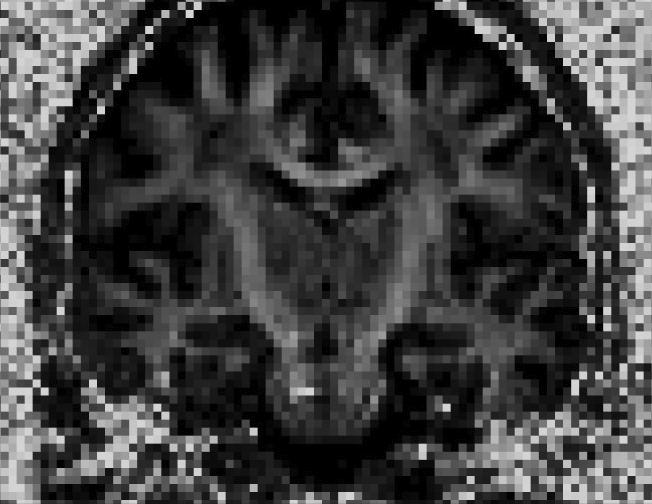
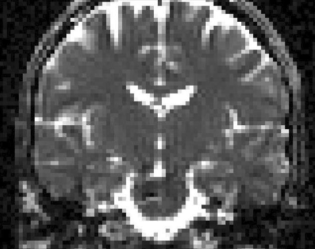
After running the dt_recon command and confirming the diffusion data is registered with the anatomical data, you may want to look at some of the outputs in Freeview. For example, you could run the following command to view the fractional anisotropy volume (fa.nii) and the apparent diffusion coefficient volume (adc.nii). The '$TUTORIAL_DIR' and '$subj' parameters need to be defined in advance. If you haven't done this already, please see the Tutorial Data Set section above.

freeview -v fa.nii adc.nii

Scroll the middle mouse button to zoom in and out. Click and hold the middle mouse button to move around the image. Use the 'Up' and 'Down' arrows (or 'Page Up' and 'Page Down' keys) to move back and forth through the volume slices. Use the orientation buttons to switch the plane ( FreeviewGuide/FreeviewGeneralUsage/FreeviewQuickStart/view_sagittal.gif , , , ). Toggle between the two volumes by using 'Alt + C'.

Coronal view of the fractional anisotropy volume (fa.nii):

Coronal view of the apparent diffusion coefficient volume (adc.nii):

All other volumetric data sets generated by dt_recon may be viewed with Freeview. To see an explanation of the various outputs, see the dt_recon page. Close Freeview when you are done before proceeding to the next step.

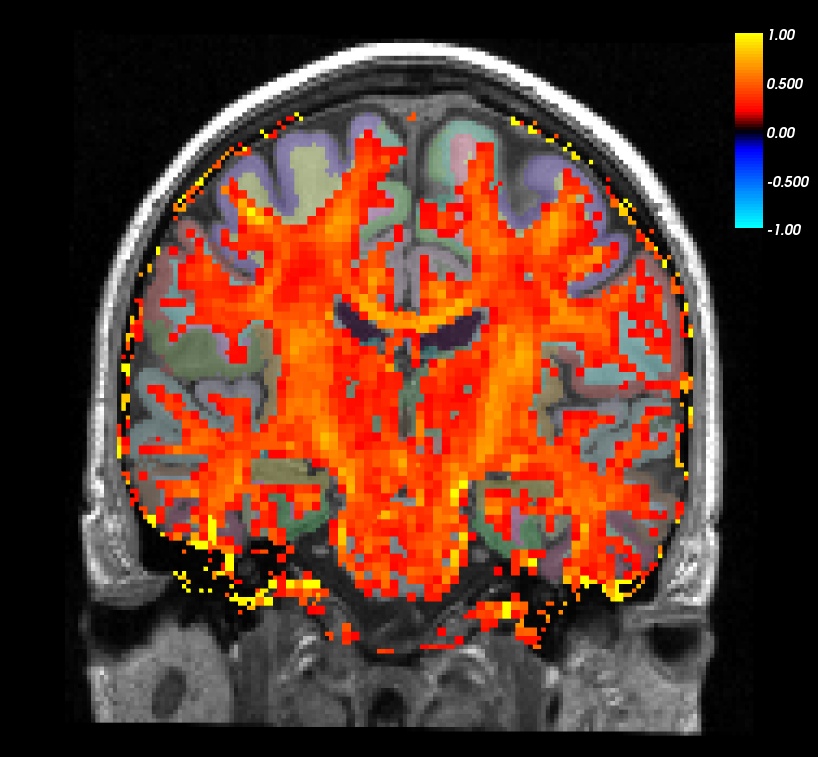
The FA map can also be viewed as a heatmap on the subject's anatomical data with the white matter parcellation (wmparc.mgz) as the segmentation, allowing you to see the FA values in various wm ROIs. While grayscale is the most common way to display FA maps, some find it easier to see the variations in FA values in a heatscale map, rather than gray scale one:

*NOTE: You must close the open Freeview window (visualizing the adc and fa maps), before you can open another one from the same terminal.

freeview -v $SUBJECTS_DIR/$subj/mri/brain.mgz \
            $SUBJECTS_DIR/$subj/mri/orig.mgz \
            $SUBJECTS_DIR/$subj/mri/wmparc.mgz:colormap=lut:opacity=0.2 \
            fa.nii:reg=register.dat:colormap=heat:heatscale=.2,.2,1 -colorscale -viewport coronal

Notes:

The FA is a value between 0 and 1, so the thresholds are set to 0.2 and 1.
When the window first comes up, there will be a lot of activity outside the brain. To remove this, with the FA volume selected, set the Mask drop-down menu to brain. This makes Freeview only show the voxels of fa.nii that coincide with voxels x > 0 on brain.mgz - everything else will disappear. This way any voxels from fa.nii outside the brain (determined by brain.mgz) will be excluded.
In the image below, you can see that white matter tends to have a higher FA.

Close Freeview when you are done. The next section shows you how to extract these FA values for each wmparc label.

Resampling Structural Data in the Diffusion Space

In order to analyze specific sub-cortical or white matter regions in the diffusion data, we can resample the subcortical segmentations created by recon-all from the structural data into the diffusion space. The registration between the diffusion and structural space has already been computed when you ran the dt_recon command above. The registration can be found in the 'register.dat' file.

The 'register.dat' file describes a rigid-body transformation from the diffusion to the structural space. But to resample the structural volume into the diffusion space, we will need to apply the inverse of this transformation to our input volumes. We use the 'mri_vol2vol' command for this task. In the example below, we resample the white-matter parcellation volume (wmparc.mgz) into the diffusion space. Additionally, you may also want to repeat that process for the cortically-labeled volume (aparc+aseg.mgz) but that is not necessary for this tutorial.

mri_vol2vol --mov lowb.nii \
            --targ $SUBJECTS_DIR/$subj/mri/wmparc.mgz \
            --inv --interp nearest --o $SUBJECTS_DIR/$subj/mri/wmparc2diff.mgz \
            --reg register.dat --no-save-reg

Notes:

The target of the original registration was in the structural space and that is indicated by the '--targ' flag. As it is the wmparc.mgz volume from the structural space that we wish to resample in the diffusion space, in the above, we identify the target volume to be just that.
The '--mov' and '--targ' input flags used should reflect the original direction of the transformation in the 'register.dat' file. We put ("moved") diffusion data into structural space. But now, we are going to put structural data into diffusion space. Thus, the role of the 'moving' and 'target' volumes are going to be inverted. It is the '--inv' flag that will reverse their roles.
When we originally computed the 'register.dat' transformation, it was the 'lowb.nii' volume that was moved into the structural space, so we indicate this volume by the '--mov' flag. (Note: any diffusion-related volume from the dt_recon outputs could be used here.)
The '--interp' flag indicates the type of interpolation that we want to use for the resampling. In the case of segmentation volumes, that option should always be set to nearest, indicating nearest neighbor interpolation.
The '--o' flag indicates the desired output filename location, which in our example is 'wmparc2diff.mgz'. The typical naming convention used is "orig2targ.mgz".
The rigid-body transformation matrix is stored in the 'register.dat' file and it is indicated by the '--reg' flag. You can use the same 'register.dat' file to move other structural volumes of this subject into the same diffusion space.
The '--no-save-reg' flag tells 'mri_vol2vol' not to write out another registration matrix file.
To see a script which could be used to run the mri_vol2vol command on multiple subjects using both the wmparc.mgz and aparc+aseg.mgz, take a look at the AlignAnat2Diff.csh script on this page.

As always, check the registration with the template. In this case, the template is the low-b image:

freeview -v lowb.nii \
            $SUBJECTS_DIR/$subj/mri/wmparc2diff.mgz:colormap=lut \
         -f $SUBJECTS_DIR/$subj/surf/lh.white:edgecolor=green \
            $SUBJECTS_DIR/$subj/surf/rh.white:edgecolor=green \
         -viewport coronal

Use Alt+V to toggle between the low-b and the wmparc, using the surfaces as a guide to make sure they are aligned.

The registration should be accurate. For more information on registration, see the Registration Tutorial.

Close Freeview when you are done.

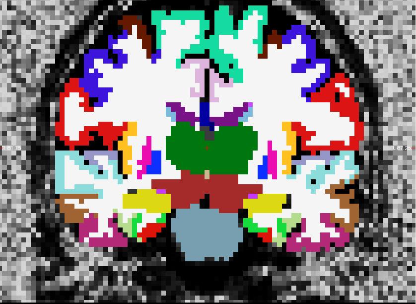
The AlignAnat2Diff.csh script mentioned above also resamples the aparc+aseg for the same subject. To view the results, run:

freeview -v fa.nii \
            $SUBJECTS_DIR/$subj/mri/aparc+aseg2diff.mgz:colormap=lut

Notes:

The resampled aparc+aseg volume is called aparc+aseg2diff.mgz.
The command above loads the resampled aparc+aseg as well as the FA volume (fa.nii) into Freeview.
To be able to see the color labels on the aparc+aseg2diff.mgz, you must specify a color table that has those labels, colors, and names. This is done with :colormap=lut attached to the volume name that the table is needed for. 'lut' stands for look-up table.

Coronal view of the cortically-labelled volume (aparc+aseg2diff.mgz) overlayed on the fractional anistropy volume (fa.nii):

Be sure to close Freeview before proceeding to the next step.

Masking

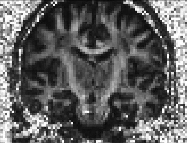
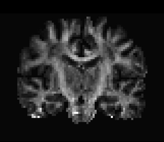
You may have noticed that there is some unwanted "noise" or "speckles" in the diffusion images when we view them in Freeview. This can be removed by masking out the space surrounding the brain. For a mask, we will use one of the segmentation volumes from the recon directory that was already resampled into the diffusion space (wmparc2diff.mgz). To apply the mask to the diffusion data and remove the unwanted "noise", we will use the 'mri_mask' command.

mri_mask fa.nii \
         $SUBJECTS_DIR/$subj/mri/wmparc2diff.mgz \
         fa-masked.mgz

Notes:

The order of the command arguments determines the action taken. The first argument should be the volume you wish to mask. The second argument is the volume to be used as a mask. And the third argument should be the name of the output file you would like to be created. In this example, we append '-masked' to the name of the original unmasked volume file so we can tell them apart.
The command above applies a mask to the fractional anisotropy volume (fa.nii), but you may run 'mri_mask' on any other diffusion volume (i.e., adc.nii, ivc.nii)
All non-brain areas will be assigned to the background.
To see a script which could be used to run the mri_mask command on multiple subjects take a look at the 'DiffMasking.csh' script on this page.
Any problems in the mask will likely be due to registration issues between the wmparc2diff.mgz and fa.nii volumes. If you want to improve the accuracy of the mask, try fixing the registration between these two volumes or add "padding" to the mask- increase the boundary of the mask by one voxel in each direction using the mri_mask -bb flag.

Run the freeview command below to compare the fractional anisotropy volume (fa.nii) before and after masking:

freeview -v fa.nii \
            fa-masked.mgz

Use Alt+c to quickly alternate between the two volumes and see the difference.

Coronal view of the unmasked fractional anisotropy volume (fa.nii):

Coronal view of the masked fractional anisotropy volume (fa-masked.mgz):

Be sure to close the Freeview window before proceeding with the next step.

FA ROI Analysis

We have already resampled the white-matter parcellation and subcortical segmentation into the subject's diffusion space. We will now use mri_segstats to get FA statistics for each of the following ROIs (index/name pairs are found in the LUT):

 251 CC_Posterior (Posterior Corpus Callosum)
3024 wm-lh-precentral
3030 wm-lh-superiortemporal
3021 wm-lh-pericalcarine
  12 Left-Putamen
   4 Left-Lateral-Ventricle

The wm-lh-precentral, wm-lh-superiortemporal, and wm-lh-pericalcarine are created by the gyral white matter parcellation. Now run mri_segstats:

mri_segstats \
    --seg $SUBJECTS_DIR/$subj/mri/wmparc2diff.mgz \
    --ctab $FREESURFER_HOME/FreeSurferColorLUT.txt \
    --id 251 --id 3021 --id 3024 --id 3030 --id 12 --id 4 \
    --i fa.nii --sum fa.stats

Click here to see the output, or open the fa.stats file in a text editor (it should be located in the directory you are currently in). You'll find the CC has an average FA of about 0.59; gyral parcellations are between 0.2-0.5; the left putamen is about 0.24; and the ventricle is about 0.12. This is as expected because the CC is highly directional with no crossing fibers so we would expect the CC to have the highest FA. The gyral white matter is also directional but has fibers crossing in them, so one expects the FA to be lower than the CC. The gray matter (putamen) is still lower. Diffusion in the ventricle is isotropic, so we expect the ventricle to have the lowest FA.

Note: ROI analysis is only as accurate as your segmentation volumes. If your segmentation volumes resampled to diffusion space are not accurate, your ROI statistics will not be accurate either. Make sure to always check your registration for mismatch between the structural and diffusion volumes. If there is no registration problem, check to make sure your segmentations in structural space are accurate.

Spatial Normalization

At this point we could run analyses on an individual subject's diffusion and structural data, but we could not do a voxel-based group analysis with multiple subjects, because the data sets are not yet aligned in a common coordinate space. In other words, a certain coordinate location in one subject's volume does not necessarily correspond to the same anatomical location in any of our other subjects. We want to normalize (resample) the diffusion data of each subject into a specified common coordinate space.

In the example below, the data will be resampled into CVS (Combined Volume and Surface registration algorithm) space, but alternatively you could normalize your data in any other coordinate system (for example, MNI or Talairach). As a result of running mri_cvs_register on the structural acquisitions, a .m3z morph file ('combined_tocvs_avg35_elreg_afteraseg-norm.m3z') is created which describes the transformation for each subject that is necessary to move from an individual's native space to that of the common CVS space. We have already run mri_cvs_register to generate the .m3z morph file for you. For more information on running mri_cvs_register on your own, click here

Don't run this command if you're at an organized course.

This command currently requires greater than 4GB of memory to run. We have already run it for you.

mri_vol2vol --targ $FREESURFER_HOME/subjects/cvs_avg35/mri/norm.mgz \
            --m3z $SUBJECTS_DIR/$subj/cvs/combined_tocvs_avg35_elreg_afteraseg-norm.m3z \
            --noDefM3zPath \
            --reg $TUTORIAL_DIR/$subj/dtrecon/register.dat \
            --mov fa-masked.mgz \
            --o fa-masked.ANAT+CVS-to-avg35.mgz \
            --interp trilin --no-save-reg

Notes:

The '--targ' flag indicates the target CVS space where we want to resample our moving volume.
The '--m3z' flag indicates the name of a morph file created for this subject by the mri_cvs_register command, which serves as a link between this subject's native space and the CVS space.
The '--noDefM3zPath' flag indicates to mri_vol2vol not to search for the morph in a default directory ($SUBJECTS_DIR/$subj/mri/transforms) but to instead use the full input filename.
The '--reg' flag identifies the rigid-body motion that describes the connection between the structural and the diffusion spaces. As the CVS morph is computed using structural volumes and in the above example we are applying the CVS morph to a diffusion volume, we need to make sure that the transformation between these two spaces (structural and diffusion, not CVS space vs. individual space) is also taken into account during the resampling process.
The '--mov' flag indicates the moving volume, the volume we want to resample in the common CVS space for a subsequent group analysis.
The '--o' flag describes the desired name of the output file.
The '--interp' flag indicates the type of interpolation we want to use for our resampling. We are not using a segmented volume as an input so we use the default trilinear (trilin) interpolation option. If you wanted to resample a segmentation volume (such as wmparc or aseg) in CVS space, you would want to use the nearest neighbor (nearest) interpolation option.
Again, the '--no-save-reg' flag tells the command not to write out another copy of the registration matrix that is being applied.
You would need to run this command on every subject in your data set before running a group analysis. To see a script which could be used to do that, take a look at the AlignAnatCVSToAVG.csh script on this page.

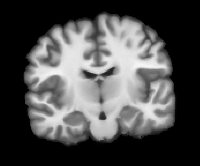
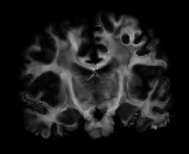
To view the 'norm.mgz' file (which is in the target CVS space) and the 'fa-masked.mgz' file after it has been resampled in the common CVS space, run:

freeview -v $FREESURFER_HOME/subjects/cvs_avg35/mri/norm.mgz \
            fa-masked.ANAT+CVS-to-avg35.mgz

Use Alt+c to alternate between the two volumes.

Coronal view of the target CVS space (norm.mgz) we resampled into:

Coronal view of the masked fractional anisotropy volume after it was resampled into CVS space (fa-masked.ANAT+CVS-to-avg35.mgz):

Once all the subjects in your study are put into the same coordinate system, you are ready to begin your group analysis on the resampled subjects.

Links Of Interest

TrackVis

Acknowledgements

dMRI tutorial scripts created by Lilla Zollei.

Quiz

You can test your knowledge of this tutorial by clicking here for a quiz!

Frequently Asked Questions

Why do we use nearest-neighbor registration with segmented volumes but trilinear registration with everything else?

Segmentation volumes have discrete values associated with them and therefore nearest-neighbor registration is used since nearest neighbor uses the actual values of the neighboring voxels for interpolation whereas trilinear registration takes an average of the surrounding voxels. Using trilinear would change the voxels values to no longer match with the segmentation label values.

Back to list of all tutorials
Back to course page