• FsTutorial
• LongitudinalTutorial

Back to list of all tutorials
Back to course page

Longitudinal Tutorial (FreeSurfer Version 6.0)

This page will take you through the steps of processing your longitudinal data:

After the tutorial (if you want to learn more) you can read details about the longitudinal stream at LongitudinalProcessing, LongitudinalEdits and LongitudinalStatistics.

---

1. Preparations

If you are taking one of the formally organized courses, everything has been set up for you on the provided laptop. The only thing you will need to do is run the following commands in every new terminal window (aka shell) you open throughout this tutorial. Copy and paste the commands below to get started:

export SUBJECTS_DIR=$TUTORIAL_DATA/long-tutorial
cd $SUBJECTS_DIR

To copy: Highlight the command in the box above, right click and select copy (or use keyboard shortcut Ctrl+c), then use the middle button of your mouse to click inside the terminal window to paste the command (or use keyboard shortcut Ctrl+Shift+v). Press enter to run the command.

These two commands set the SUBJECTS_DIR variable to the directory where the data is stored and then navigates into this directory.

If you are NOT taking one of the formally organized courses, click here.

---

2. Longitudinal Image Processing

All data for this tutorial has already been processed for you since processing can take up to 24h. However, to continue you need to understand the three processing steps (cross, base, long) and associated directory names.

For example, assume you have a subject with two time points: OAS2_0001_MR1 and OAS2_0001_MR2.

1. [CROSS]: You would process these two images independently first (we call that cross as in crossectional analysis/processing) using the regular FreeSurfer processing stream (recon-all). You end up with two directories with the names OAS2_0001_MR1 and OAS2_0001_MR2

2. [BASE]: Then you would run the second step to create the within subject template (also called base) and end up with a new directory. There is only one base directory per subject. We decide to name the base: OAS2_0001. Inside this directory are the results for the average anatomy of your subject across time. You don't use this data in any analysis, and only look at it for quality checking or editing.

3. [LONG]: Finally you would create the two longitudinal runs (the ones you are actually interested in). You end up with two more directories (these names get automatically assigned): OAS2_0001_MR1.long.OAS2_0001 and OAS2_0001_MR2.long.OAS2_0001. They contain the final, most reliable and accurate processing results.

For the subjects described above, the commands for creating the cross, base, and long are the following. For a subject with two time points OAS2_0001_MR1 and OAS2_0001_MR2 you would run the independent runs first by typing (don't do it, it has already been done for you) in two separate terminals or on different computers:

recon-all -subjid OAS2_0001_MR1 -all

recon-all -subjid OAS2_0001_MR2 -all

If you work with your own data, you'd have to import the dicoms first recon-all -i path_to_your_dcm1 ... -subjid your_subject_name. In this command you can pass several within-session scans by specifying multiple -i flags instead of the "...". You then run the above recon-all comands to process the imported data. We call these runs the cross sectionals (or cross runs) because the two time points are processed completely independently as if they were from different subjects.

Once the norm.mgz is available on both time points, you can create the unbiased subject template/base (don't do it, it has already been done for you). We decide to name it OAS2_0001 :

recon-all -base OAS2_0001 -tp OAS2_0001_MR1 -tp OAS2_0001_MR2 -all

This will create the within-subject template (we will refer to these type of runs as base) and run it through recon-all. It will take approximately the same time as a regular recon-all run, a little more because of the initial averaging of time points. A directory OAS2_0001 will be created.

Finally once the base and the two cross sectionally processed time points are fully completed, you can run the longitudinal runs (again in two different terminals or different computers) by typing:

recon-all -long OAS2_0001_MR1 OAS2_0001 -all

recon-all -long OAS2_0001_MR2 OAS2_0001 -all

These runs create the directories OAS2_0001_MR1.long.OAS2_0001 and OAS2_0001_MR2.long.OAS2_0001 containing the final results. These are complete subjects directories and we will use them for any post-processing or analysis as the results are more sensitive and repeatable than the independent cross runs. These longitudinal processes run much faster than the cross and base above. We call them the longitudinal or simply long runs, because they make use of common information taken from the template.

You can now continue with the next section (inspecting the data).

If you want to learn about the exact commands for processing your data, click here.

---

3. Inspecting Longitudinal Data

We use freeview (FreeviewGuide) as a viewer in this tutorial.

First let's check the base (subject template) of a single subject. Open the norm.mgz and surfaces with freeview. If you run the following command and freeview opens, switch to the coronal view in order to see the same as the images below:

freeview -v OAS2_0001/mri/norm.mgz \
         -f OAS2_0001/surf/lh.pial:edgecolor=red \
            OAS2_0001/surf/rh.pial:edgecolor=red \
            OAS2_0001/surf/lh.white:edgecolor=blue \
            OAS2_0001/surf/rh.white:edgecolor=blue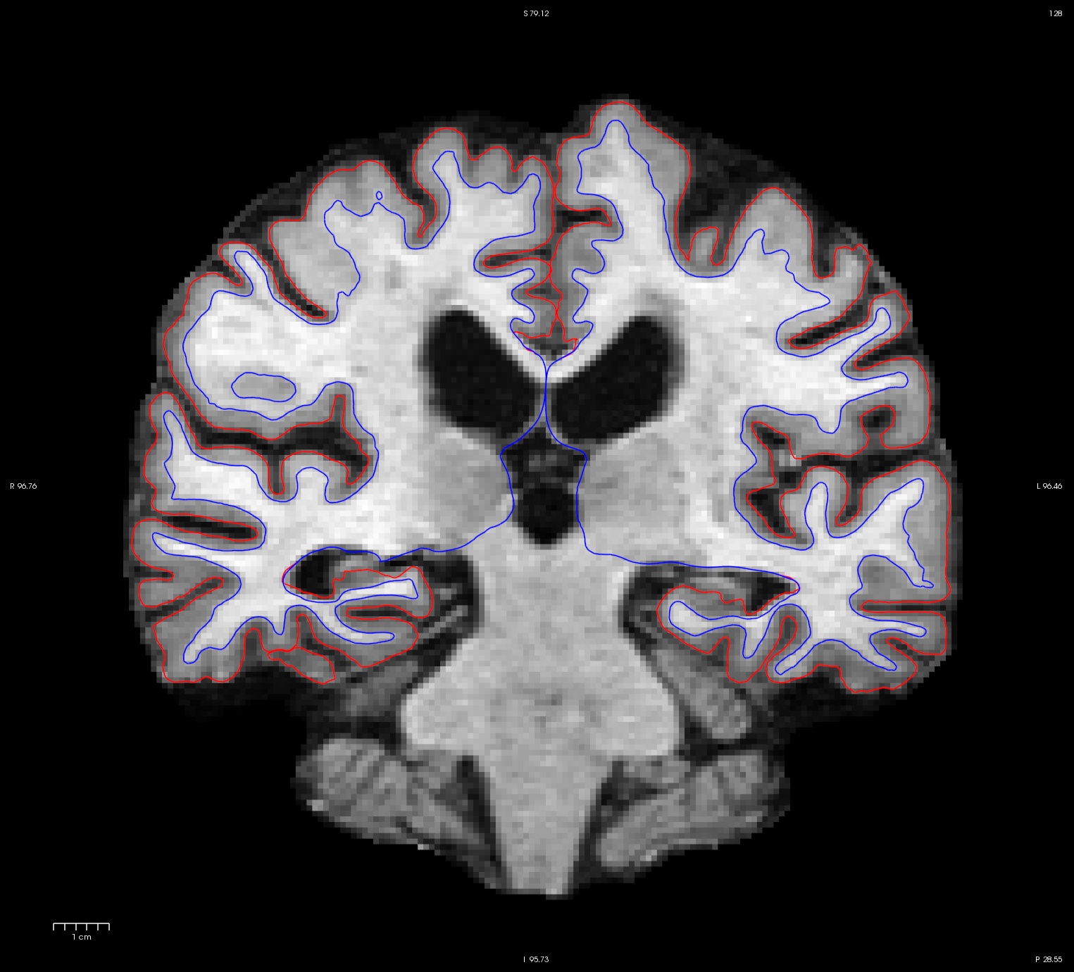

This will show you the within-subject template (base), i.e., the average anatomy of this subject across time overlayed with the pial and white surface. If the across-time registration failed you would see a blurry image or ghosting. You should inspect the surfaces on this image. This will be important later as the surfaces are transferred into the longitudinal runs and therefore should be accurate in the base. Move back and forth to inspect all slices and see if the surfaces follow the white matter and gray matter boundaries.

Now it is time to look at the longitudinal results. Starting with FreeSurfer 5.1, the base and the long volumes are all in the same voxel space, meaning that volumes across time are anatomically aligned and can be directly compared if opened on top of each other ). Close any open freeview window to reduce memory usage and run the following command:

freeview -v OAS2_0001_MR1.long.OAS2_0001/mri/norm.mgz \
            OAS2_0001_MR2.long.OAS2_0001/mri/norm.mgz \
         -f OAS2_0001_MR1.long.OAS2_0001/surf/lh.pial:edgecolor=red \
            OAS2_0001_MR1.long.OAS2_0001/surf/lh.white:edgecolor=blue \
            OAS2_0001_MR2.long.OAS2_0001/surf/lh.pial:edgecolor=255,128,128 \
            OAS2_0001_MR2.long.OAS2_0001/surf/lh.white:edgecolor=lightblue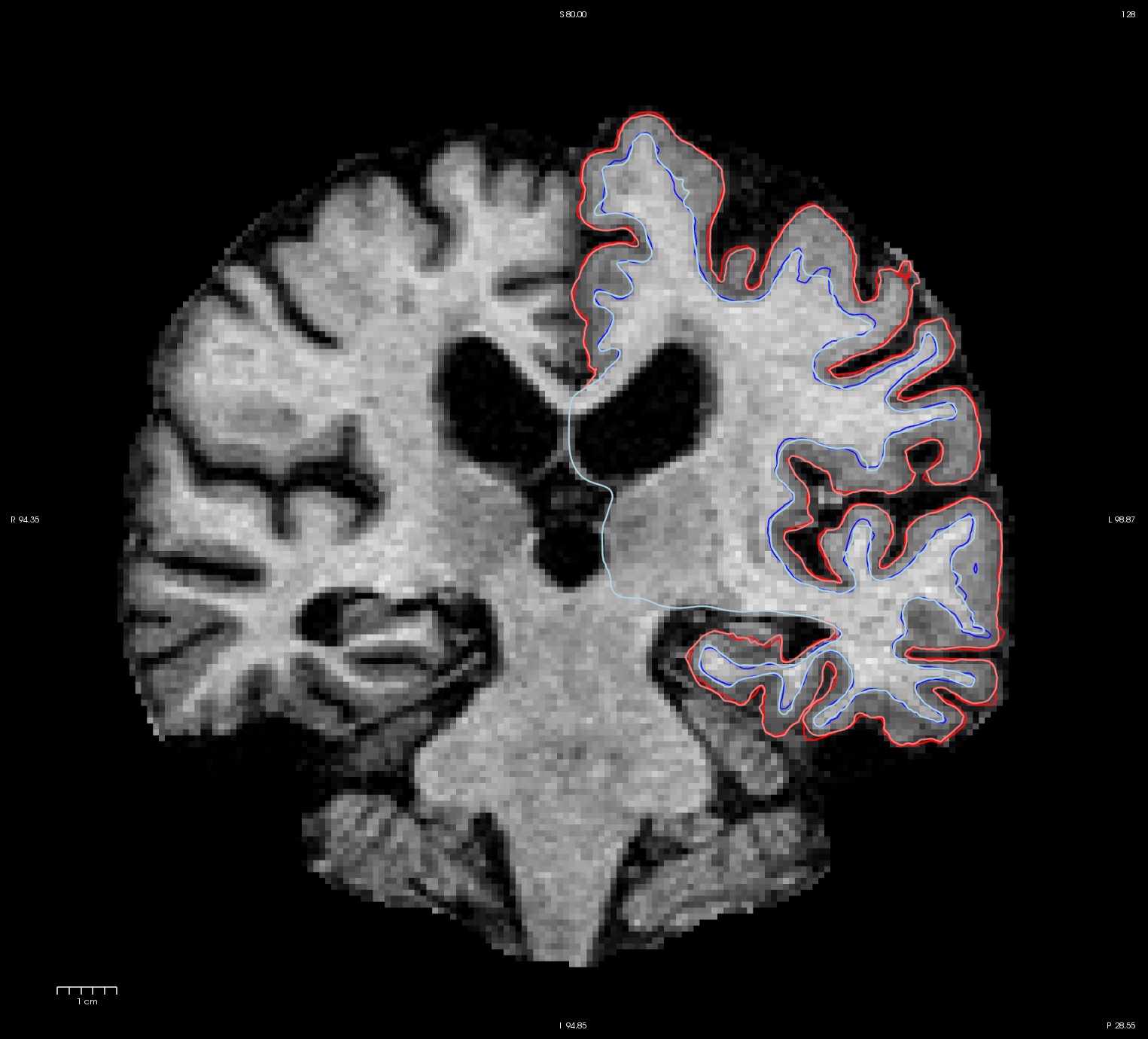

This might take a while to load (check the progress bar). You will see the normalized skull stripped images (norm.mgz) of both time points on top of each other (the second time point is the top-most layer and so the only one visible at the moment). You also see the white and pial surface for each time point, drawn on top of each other (we only show the left hemisphere here to reduce memory usage for older computers). Time point 1 uses red and blue while time point 2 uses pink and light blue for the surface colors. The surfaces do not change much across time. You can also compare the images directly. For this, uncheck the 4 check boxes in front of all the surfaces, or press 'Ctrl-f'. Select the first (top) norm volume and use the opacity slider to blend between the two images. You can also switch back and forth between the two images by pressing 'Alt-c' or using the opacity slider. This way you can spot longitudinal deformations (atrophy) and also potential global alignment problems (not in this case). You will mainly notice that the ventricles are getting larger in the second time point. You can use the Up and Down arrow keys to scroll through the slices. Close freeview when done.

---

4. Post-Processing Longitudinal Data

4.1. Longitudinal Table

(Also: LongitudinalStatistics)

To get the longitudinal data ready for the statistical analysis, you need to create a table (space separated as a text file) in the following format:

where the first column is called fsid (containing each time point) and the second column is fsid-base containing the base name, to group time points within subject. You can have many more columns such as gender, age, group, drug, etc. Make sure there is a column containing an accurate time variable (optimally measured in years if you are interested in yearly change) such as age or the duration of the study (time from initial scan). Here we use years to measure the time from baseline scan (=tp1). You can see in the table that the two subjects OAS2_0001 and OAS2_0004 each have two time points (MR1,MR2) that are not equally spaced (approx 15 and 18 months apart). We have created this table for you in the qdec subdirectory for the tutorial data and can get started right away. You can look at the file by opening it in your favourite spreadsheet editor, e.g.:

libreoffice -calc qdec/long.qdec.table.dat

or, if that fails, a simple text editor:

gedit qdec/long.qdec.table.dat

NOTE: For Mac users, you can try Numbers, Excel or a simple text editor:

open qdec/long.qdec.table.dat -a Numbers

open qdec/long.qdec.table.dat -a "Microsoft Excel"

open -e qdec/long.qdec.table.dat

4.2. What kind of statistical analysis to perform?

FreeSurfer offers different ways to analyze longitudinal data (details: LongitudinalStatistics). The GLM group analysis tutorials teach you how to run some simple statistical analyses on thickness maps (e.g. to find cortical regions with different thickness across groups). In this tutorial we will describe how to get your longitudinal data ready for statistical analysis, but not to do the actual model fitting.

The two most frequently used models are the simple two-stage model (LongitudinalTwoStageModel) and a fully flexible mixed effects model (LinearMixedEffectsModels) (LME), which is recommended for statistical analysis but requires Matlab knowledge. LME can, for example, deal with different time deltas and time points, missing data, and include subjects with only a single time point. The 2-stage model on the other hand, first performs a linear fit in each subject independently to reduce the repeated measures to a single number (slope, such as mm/year) and then performs a regular cross sectional analysis across subjects (e.g. to look for age or group effects).

Users who are interested in preparing data for the more powerful and complex mixed effects modeling can see how it is done by clicking here.

In this tutorial, we will prepare the data for a simple statistical model for longitudinal data, consisting of two stages:

1. We reduce repeated measures to a single number for each subject. For example, quantifying atrophy rates (as mm/year thinning or percent change).
2. This measure can then be compared across groups (e.g. with a standard glm_fit analysis) to detect disease or treatment effects.

4.3. Preparing the Thickness Data - QCACHE

The following command can be used to prepare the data:

long_mris_slopes --qdec ./qdec/long.qdec.table.dat --meas thickness --hemi lh --do-avg --do-rate --do-pc1 --do-spc --do-stack --do-label --time years --qcache fsaverage --sd $SUBJECTS_DIR

This will:

• (--qdec) read in the table
• (--meas thickness) take the thickness measure of each time point
• (--hemi) specify which hemisphere to work on (here 'lh' specified)
• (--do-avg) compute the temporal average (thickness at midpoint of linear fit, here it is just the average)
• (--do-rate) compute the rate of change (thickening in mm/year)
• (--do-pc1) compute the percent change (with respect to time point 1)
• (--do-spc) compute a symmetrized percent change (with respect to the temporal average)
• (--do-stack) output a stacked thickness file for each subject (time series)
• (--do-label) intersect the cortex label to ensure we don't include non-cortex regions
• (--time) specify the column in the longqdec.table.dat that contains the time variable (here 'years' specified)
• (--qcache) and automatically smooth everything on different levels and map it to fsaverage (note how this is specified after the flag)
• (--sd) specify the subject directory (needs to be passed explicitly since FS 5.2)

We pass all these parameters as an example. Usually you will not compute the average, select rate, pc1 or spc (depending on what you are interested in) and not explicitly write out the stack which is used for debugging (so drop --do-avg and --do-stack and select from --do-rate, --do-pc1 or do-spc). You then need to run the same command for the right hemisphere (--hemi rh).

(Note, if you split your table up into smaller tables containing only information for a specific subject each, you can run this on a cluster in parallel for each subject to speed things up (you can use the commands below to split the table up into individual subjects inside the qdec directory).

cd qdec
long_qdec_table --qdec ./long.qdec.table.dat --split fsid-base
cd ..

Now before continuing, let's get an idea about what the above four measures mean in our setting (with only two time points):

1. The temporal average is simply the average thickness: avg = 0.5 * (thick1 + thick2), usually you don't want to analyse this, as you are mainly interested in change.

2. The rate of change is the difference per time unit, so rate = ( thick2 - thick1 ) / (time2 - time1), here thickening in mm/year. In aging or disease we expect it to be negative in most regions (because of noise not necessarily for a single subject, but on average). For more than two time points, this is the slope of the linear fit.

3. The percent change (pc1) is the rate with respect to the thickness at the first time point: pc1 = rate / thick1. We also expect it to be negative and it tells how much percent thinning we have at a given cortical location.

4. The symmetrized percent change (spc) is the rate with respect to the average thickness: spc = rate / avg. This is a more robust measure than pc1, because thickness at time point 1 is more noisy than the average. Also spc is symmetric: when reversing the order of tp1 and tp2 it switches sign. This is not true for pc1. Therefore, and for other reasons related to increased statistical power, we recommend to use spc.

So let's investigate (some of) the results, which can be found in each base surf directory. Call this to open up the pial surface (left hemi) of subject OAS2_0001:

freeview -f OAS2_0001/surf/lh.pial:overlay=OAS2_0001/surf/lh.long.thickness-avg.fwhm15.mgh:overlay_threshold=0,3.5:overlay=OAS2_0001/surf/lh.long.thickness-stack.mgh:annot=OAS2_0001/label/lh.aparc.annot:annot_outline=1 --timecourse --colorscale --viewport 3d

Click on the 3D view button if freeview opens in a different view from what is depicted in the screenshot below, then click somewhere on the cortex to see the time course data at that location.

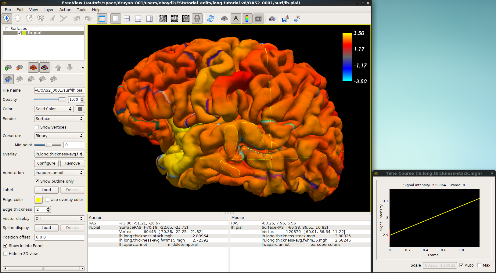
You are looking at the smoothed average thickness (color overlay) with values between 1 (red) and >3 mm (yellow). If you click at any location on the surface you can see a plot of the two original (unsmoothed) thickness values at the two time points. We also opened the cortical parcellation (aparc, using the annot flag) in outline style, which can be switched on and off. It helps to find out what region you are inspecting when clicking on the surface. For a single subject values are often noisy even after smoothing and show local thinning and thickening. That is why for a group analysis one needs several subjects in each group. The yellow lines/curves in the main window on the surface show the intersection of the three planes with the cortex at the selected location, and can be ignored.

For users with only an older Freeview version (no support for time course), you can use tksurfer to achieve the same (no need to do it in the course):

tksurfer OAS2_0001 lh pial -overlay $SUBJECTS_DIR/OAS2_0001/surf/lh.long.thickness-avg.fwhm15.mgh -timecourse $SUBJECTS_DIR/OAS2_0001/surf/lh.long.thickness-stack.mgh -aparc

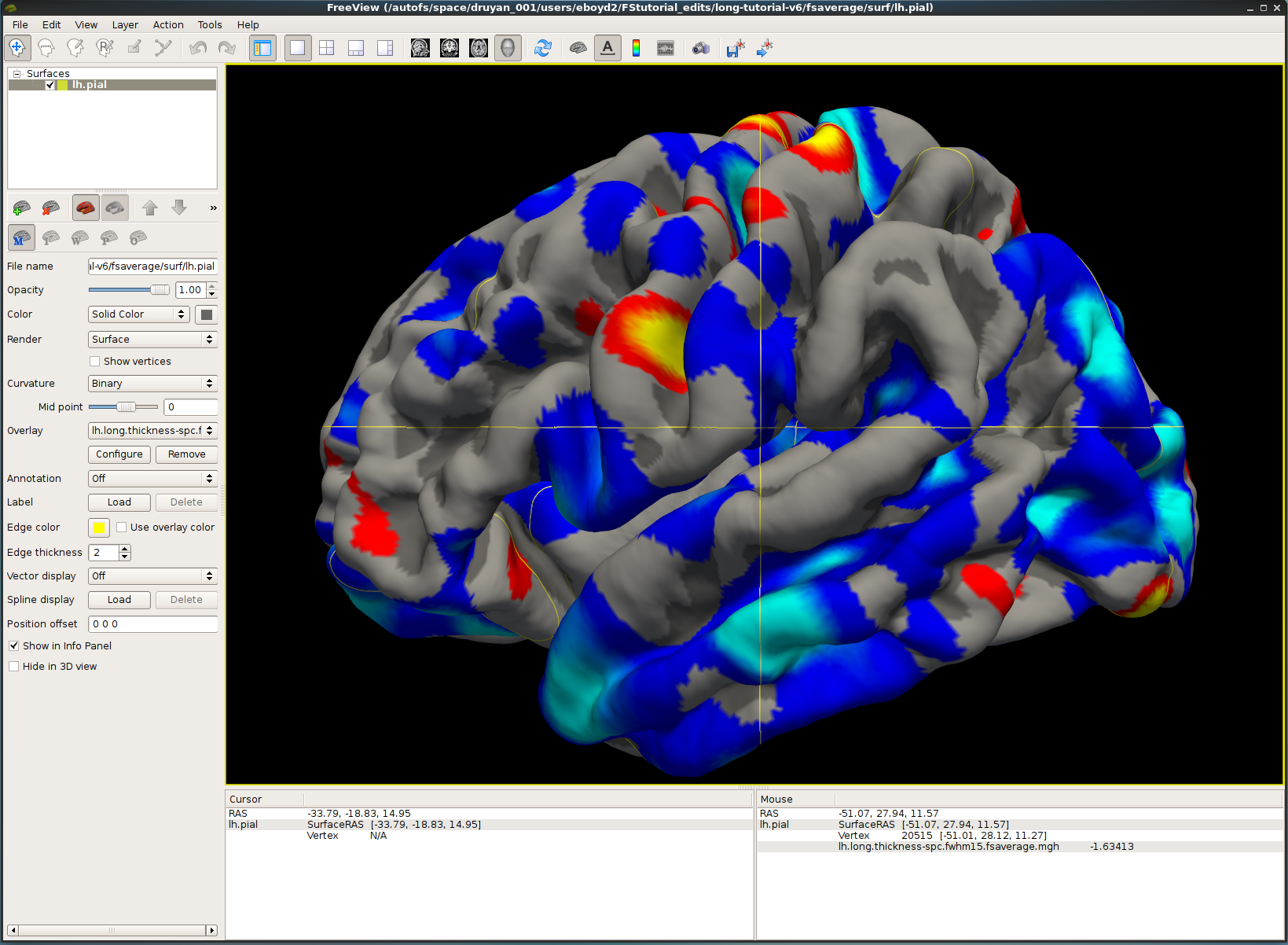
In a similar fashion, you can open, for example, the symmetrized percent change. Close any open freeview windows. This time we open the overlay on fsaverage, an average subject provided with FreeSurfer and often used as the common target to compare results across subjects. The --qcache flag of long_mris_slopes has conveniently registered and mapped all results to this average subject:

freeview -f $FREESURFER_HOME/subjects/fsaverage/surf/lh.pial:overlay=$SUBJECTS_DIR/OAS2_0001/surf/lh.long.thickness-spc.fwhm15.fsaverage.mgh:overlay_threshold=2,5

note the 'fsaverage' in the filename. Because there is not much change on the surfaces, the SPC will be even more noisy than the average. You can use the above commands to investigate individual results, but this is rarely necessary.

Since FS5.2: Similar to the long_mris_slopes command above to compute thickness change, you can use long_stats_slopes to compute subject rates, percent changes, etc. for the ROI stats (aseg or aparc, i.e. subcortical and cortical ROI volumes and average thickness). Once you reduced the measures to a single number per subject, you can compare groups similar to a cross sectional analysis (e.g. using mri_glm_fit).

Close freeview when finished.

---

5. Editing Longitudinal Data

Editing longitudinal data can be complicated, but in some cases you actually save time, as some edits are only necessary in the base. You should be familiar with Edits and might want to check also the page about LongitudinalEdits. To refresh how to perform edits using Freeview, navigate to the FreeviewGuide.

Here are some examples of some common errors you can encounter with your data. Notes: Because some of the recons take a while to run and it is not practical for you to run them during this short period of time, we ran the edits ahead of time. You will see that the edited and re-processed version have the postfix '_fixed'.

5.1. Skullstrip Error

The most common type of skull strip failures you probably will see has to do with the cerebellum: Often, part of the cerebellum is stripped off (as you have seen in the skull strip tutorial in the troubleshooting portion earlier). Sometimes skull stripping will also leave too much dura behind. For either case, the best way to solve the problem is to adjust the watershed parameters.

Very rarely, you will see FreeSurfer fail completely in the skullstrip step (usually associated with many other errors) as is clearly the case in the following example. For the purpose of this tutorial, we will only focus on and fix the skull strip error in this case.

Before starting this section, change your SUBJECTS_DIR to where the skullstrip example data is:

export SUBJECTS_DIR=$TUTORIAL_DATA/long-tutorial/skullstrip
cd $SUBJECTS_DIR

Let's take a look at the base for subject OAS2_0004:

freeview -v OAS2_0004/mri/T1.mgz \
            OAS2_0004/mri/brainmask.mgz \
         -f OAS2_0004/surf/lh.pial:edgecolor=red \
            OAS2_0004/surf/rh.pial:edgecolor=red \
            OAS2_0004/surf/lh.white:edgecolor=blue \
            OAS2_0004/surf/rh.white:edgecolor=blue

You are looking at a completely misaligned average image in the base for this subject. In order to find out what causes these problems, it is important to also check the cross-sectional runs for the same subject to see if the problem is present there. While looking at the base helps to see that this subject's processing has a problem, you should always check to see whether the initial cross sectional processing already fails.

You can open the cross subjects with the commands below. NOTE: We suggest only opening one freeview window at a time if you are using an old computer or one without much RAM. Freeview uses a large amount of memory, and may slow down your computer.

freeview -v OAS2_0004_MR1/mri/T1.mgz \
            OAS2_0004_MR1/mri/brainmask.mgz \
         -f OAS2_0004_MR1/surf/lh.pial:edgecolor=red \
            OAS2_0004_MR1/surf/rh.pial:edgecolor=red \
            OAS2_0004_MR1/surf/lh.white:edgecolor=blue \
            OAS2_0004_MR1/surf/rh.white:edgecolor=blue

freeview -v OAS2_0004_MR2/mri/T1.mgz \
            OAS2_0004_MR2/mri/brainmask.mgz \
         -f OAS2_0004_MR2/surf/lh.pial:edgecolor=red \
            OAS2_0004_MR2/surf/rh.pial:edgecolor=red \
            OAS2_0004_MR2/surf/lh.white:edgecolor=blue \
            OAS2_0004_MR2/surf/rh.white:edgecolor=blue

These commands will open the brainmask.mgz volume, the T1.mgz, and the surfaces for both hemispheres. You can check the brainmask.mgz volume and compare it to the T1.mgz volume (use Alt+v to toggle between them).

As you can see, the skull strip for this subject is very poor for both timepoints MR1 and MR2 (cross), therefore affecting the results of the base and the longitudinals downstream. Don't be overwhelmed by other problems presented in this case. You should always find out if there is a skullstrip error first, fix that, then attack the rest of the problems. You'll be surprised how much less you'll have to go through in the end. Take it one step at a time.

5.1.1. Fixing a bad skull strip

First, take a look at the coronal slice 125 for OAS2_0004_MR1, you can see that the entire neck is still present.

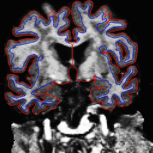
Now look at OAS2_0004_MR2. This timepoint looks even worse with parts of the skull still present and parts of the brain stripped off. If you scroll to slice 66, you will see that a great part of the brain is missing. Below is the comparison between the brainmask.mgz (left) and T1.mgz (right) for slice 66.

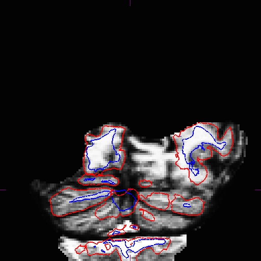
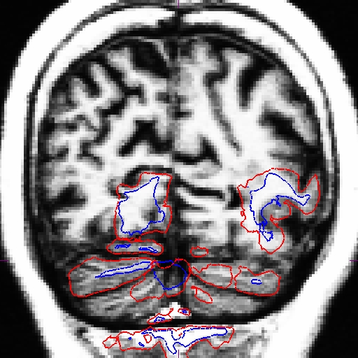
The best way to fix a problem like this is to adjust the watershed parameters. As mentioned earlier, this can only be done on the cross-sectionals, and you'll have to use the edited cross-sectionals to recreate the base and the longitudinals afterwards. Adjust the watershed parameters for both MR1 and MR2 using the following commands. Feel free to run these commands (separately) since this step is fairly quick (This command is optional).

recon-all -subjid OAS2_0004_MR1 -skullstrip -wsthresh 20 -clean-bm -no-wsgcaatlas

recon-all -subjid OAS2_0004_MR2 -skullstrip -wsthresh 55 -clean-bm -no-wsgcaatlas

For OAS2_0004_MR1, the brain is intact while a lot of the skull is left behind, therefore we decreased the watershed threshold. As for OAS2_0004_MR2, we don't want to strip away more brain so we increased the threshold. Play around with different numbers and see what you get. If you ran the commands, take a look at your output volumes (directory w/o _fixed), or simply check our edited volumes, and verify that the result of the new skull stripping is correct.

It is necessary to run the rest of the cross sectional recon-all steps for all timepoints that you made an adjustment to:

recon-all -subjid OAS2_0004_MR1 -autorecon2 -autorecon3

recon-all -subjid OAS2_0004_MR2 -autorecon2 -autorecon3

These _fixed versions were already run with -autorecon2 and -autorecon3.

freeview -v OAS2_0004_MR1_fixed/mri/T1.mgz OAS2_0004_MR1_fixed/mri/brainmask.mgz

freeview -v OAS2_0004_MR2_fixed/mri/T1.mgz OAS2_0004_MR2_fixed/mri/brainmask.mgz

To save time, you can check in with the recon-all-status.log in the scripts directory of these subjects to see if the normalization step is complete. Once that step is complete, you can start recreating your base (remove/rename the base dir if it existed, e.g. mv OAS2_0004 OAS2_0004_old, before running this). Alternatively, you can wait until the recons are complete to check whether all surfaces are updated as desired. Here are the results for OAS2_0004_MR1 slice 125 and OAS2_0004_MR2 slice 66.

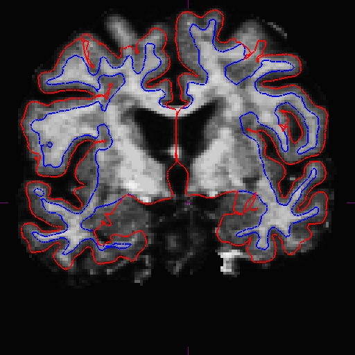
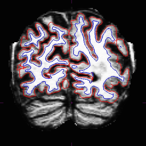
*Notice the huge improvement between OAS2_0004_MR2_fixed and the original one. You might not arrive at this output if you just ran the watershed parameter with threshold 55 and rerunning -autorecon2 -autorecon3 once.

After those initial runs, we noticed that there was still a good amount of skull left over, so we ran the following commands:

recon-all -skullstrip -subjid OAS2_0004_MR2

recon-all -autorecon2 -autorecon3 -subjid OAS2_0004_MR2

Sometimes just rerunning the -skullstrip step will help fix the problem without you having to do any extra adjustments. This is because during this step, FreeSurfer uses the existing brainmask.mgz as input and that can make a big difference on the output.

5.1.2. Recreating base and longs

Now you are ready to recreate the base.

recon-all -base OAS2_0004 -tp OAS2_0004_MR1 -tp OAS2_0004_MR2 -all

Then, the final step is to recreate the longitudinals once the base and cross sectional runs are complete:

recon-all -long OAS2_0004_MR1 OAS2_0004 -all

recon-all -long OAS2_0004_MR2 OAS2_0004 -all

**NOTE**: When recreating the base and longitudinals, it is recommended to remove or rename the existing base and longitudinal directories and start those processes from scratch, if possible.

5.1.3. Viewing final results

You can examine the corrected version of the base and longitudinals by using the following commands in separate terminals.

freeview -v OAS2_0004_fixed/mri/T1.mgz \
            OAS2_0004_fixed/mri/brainmask.mgz \
         -f OAS2_0004_fixed/surf/lh.pial:edgecolor=red \
            OAS2_0004_fixed/surf/rh.pial:edgecolor=red \
            OAS2_0004_fixed/surf/lh.white:edgecolor=blue \
            OAS2_0004_fixed/surf/rh.white:edgecolor=blue

freeview -v OAS2_0004_MR1.long.OAS2_0004_fixed/mri/T1.mgz \
            OAS2_0004_MR1.long.OAS2_0004_fixed/mri/brainmask.mgz \
         -f OAS2_0004_MR1.long.OAS2_0004_fixed/surf/lh.pial:edgecolor=red \
            OAS2_0004_MR1.long.OAS2_0004_fixed/surf/rh.pial:edgecolor=red \
            OAS2_0004_MR1.long.OAS2_0004_fixed/surf/lh.white:edgecolor=blue \
            OAS2_0004_MR1.long.OAS2_0004_fixed/surf/rh.white:edgecolor=blue

freeview -v OAS2_0004_MR2.long.OAS2_0004_fixed/mri/T1.mgz \
            OAS2_0004_MR2.long.OAS2_0004_fixed/mri/brainmask.mgz \
         -f OAS2_0004_MR2.long.OAS2_0004_fixed/surf/lh.pial:edgecolor=red \
            OAS2_0004_MR2.long.OAS2_0004_fixed/surf/rh.pial:edgecolor=red \
            OAS2_0004_MR2.long.OAS2_0004_fixed/surf/lh.white:edgecolor=blue \
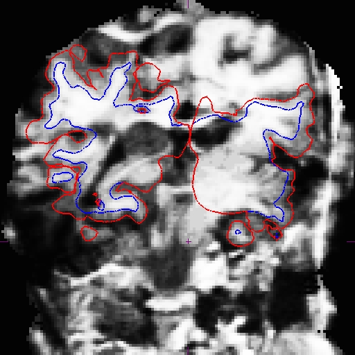
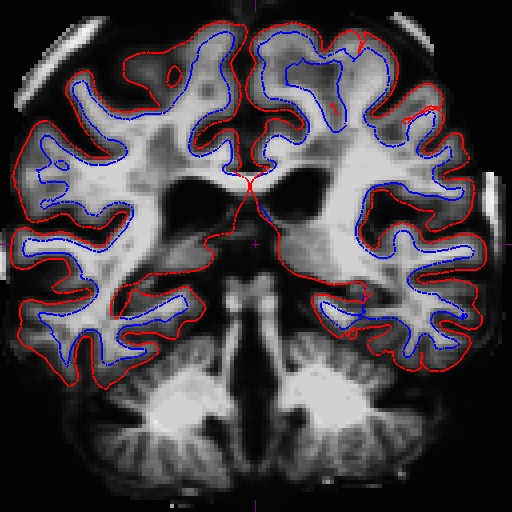
            OAS2_0004_MR2.long.OAS2_0004_fixed/surf/rh.white:edgecolor=blue

---

If you were horrified while looking at the base earlier, which is the left image at coronal slice 120 below, compare it to the right image, also at coronal slice 120, after the skullstrip fix.

And here are the longitudinals for OAS2_0004_MR2.long.OAS2_0004. Before (left) at slice 145 and after (right) at the same slice.

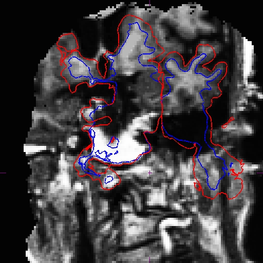
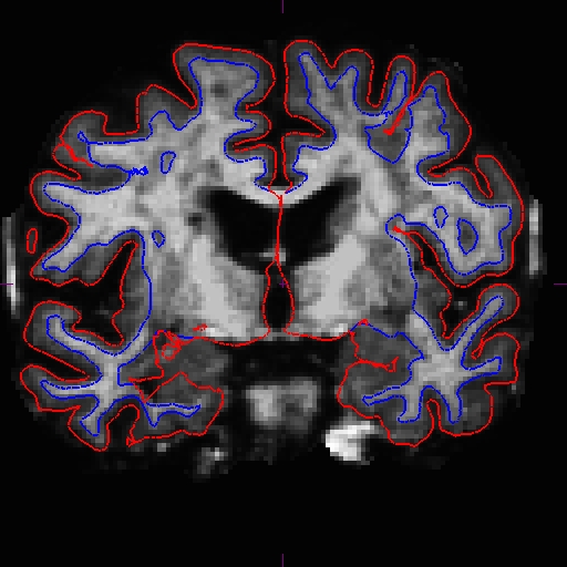
Note that, although much has been fixed, there are still problems here that need special treatment (e.g. exclusion of wm from the surfaces at various places). With these, you can start making manual edits on the wm or you can use other appropriate methods. *Take home message* - although your case might appear like this one we just went through, and you might think that it's impossible to remedy, take it one step at a time. Usually several adjustments to the skullstrip parameters can make this big of a difference.

---

For more details on skull strip errors and the different ways to fix them, refer back to the Troubleshooting Skull Strip Tutorial.

5.2. Pial/Brainmask Edits

Before starting this section, set your SUBJECTS_DIR back to the parent directory for this tutorial:

export SUBJECTS_DIR=$TUTORIAL_DATA/long-tutorial/
cd $SUBJECTS_DIR

Sometimes you will come across a case where you need to make edits to the brainmask.mgz to correct the pial surfaces. Open subject OAS2_0057 to see where and how this type of edit should be done.

First, open the base:

freeview -v OAS2_0057/mri/T1.mgz \
            OAS2_0057/mri/brainmask.mgz \
         -f OAS2_0057/surf/lh.pial:edgecolor=red \
            OAS2_0057/surf/rh.pial:edgecolor=red \
            OAS2_0057/surf/lh.white:edgecolor=blue \
            OAS2_0057/surf/rh.white:edgecolor=blue

This will open the brainmask.mgz volume, T1.mgz volume, and all surfaces. You can also check out the cross-sectionals and the longitudinals of this subject to check if the problem is present in all parts of the stream. NOTE: We suggest only opening one freeview window at a time if you are using an old computer or one without much RAM. Freeview uses a large amount of memory, and may slow down your computer.

freeview -v OAS2_0057_MR1/mri/T1.mgz \
            OAS2_0057_MR1/mri/brainmask.mgz \
         -f OAS2_0057_MR1/surf/lh.pial:edgecolor=red \
            OAS2_0057_MR1/surf/rh.pial:edgecolor=red \
            OAS2_0057_MR1/surf/lh.white:edgecolor=blue \
            OAS2_0057_MR1/surf/rh.white:edgecolor=blue

freeview -v OAS2_0057_MR2/mri/T1.mgz \
            OAS2_0057_MR2/mri/brainmask.mgz \
         -f OAS2_0057_MR2/surf/lh.pial:edgecolor=red \
            OAS2_0057_MR2/surf/rh.pial:edgecolor=red \
            OAS2_0057_MR2/surf/lh.white:edgecolor=blue \
            OAS2_0057_MR2/surf/rh.white:edgecolor=blue

freeview -v OAS2_0057_MR1.long.OAS2_0057/mri/T1.mgz \
            OAS2_0057_MR1.long.OAS2_0057/mri/brainmask.mgz \
         -f OAS2_0057_MR1.long.OAS2_0057/surf/lh.pial:edgecolor=red \
            OAS2_0057_MR1.long.OAS2_0057/surf/rh.pial:edgecolor=red \
            OAS2_0057_MR1.long.OAS2_0057/surf/lh.white:edgecolor=blue \
            OAS2_0057_MR1.long.OAS2_0057/surf/rh.white:edgecolor=blue

freeview -v OAS2_0057_MR2.long.OAS2_0057/mri/T1.mgz \
            OAS2_0057_MR2.long.OAS2_0057/mri/brainmask.mgz \
         -f OAS2_0057_MR2.long.OAS2_0057/surf/lh.pial:edgecolor=red \
            OAS2_0057_MR2.long.OAS2_0057/surf/rh.pial:edgecolor=red \
            OAS2_0057_MR2.long.OAS2_0057/surf/lh.white:edgecolor=blue \
            OAS2_0057_MR2.long.OAS2_0057/surf/rh.white:edgecolor=blue

See if you can find the slices where you will need to edit the braimask.mgz in order to correct the surfaces. Continue reading for a detailed description on how and at which stage you can fix this problem.

6. Making Pial Surfaces Edits

Towards the anterior region of the brain, notice that there's a lot of dura remaining from the skullstrip making the pial surface extend farther out from the grey matter. In these cases, manual edits will be the quickest way to fix the problem. Also notice that this problem exists in all three stages: cross, base, and long. Except for very special cases (e.g. comparing cross sectional vs. longitudinal processing) you will not need the final cross-sectional results, but instead use the longitudinal results for downstream analysis. Therefore, it is easiest and quickest now to just edit the base, and then rerun the base and longitudinal data from there. If you prefer to correct the cross-sectionals, you can also do that, the base should automatically be fixed, but needs to be checked.

Remember to delete the base directory when you are recreating a new base from your edited cross time points, or at least delete the brainmask.mgz file from the mri directory of the base before rerunning it, to make sure that the updates are transferred.

The following are before images from the base OAS2_0057 coronal slices 174 and 203, respectively.

---

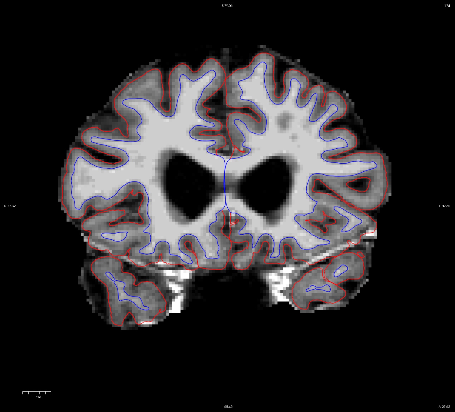
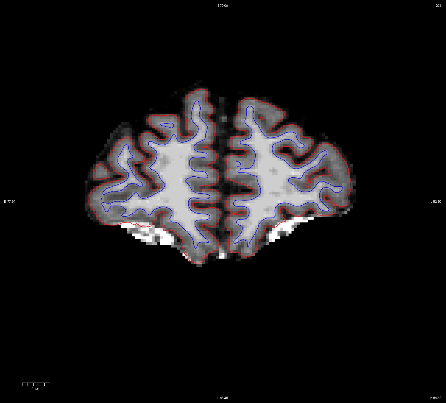
We will step through the quick route of just editing the base. After deleting the extra dura from brainmask.mgz, rerun the base with the following command:

recon-all -base OAS2_0057 -autorecon-pial

To rerun the longitudinals, use the following commands (note - it is better if you delete or rename the existing longitudinal directories for this subject. Or you can delete the brainmask.mgz in the mri directories if you don't want to delete the whole subjectdir, maybe because of other edits in the long runs.)

recon-all -long OAS2_0057_MR1 OAS2_0057 -all

recon-all -long OAS2_0057_MR2 OAS2_0057 -all

---

Here is the final output of the base for the same coronal slices, 174 and 203:

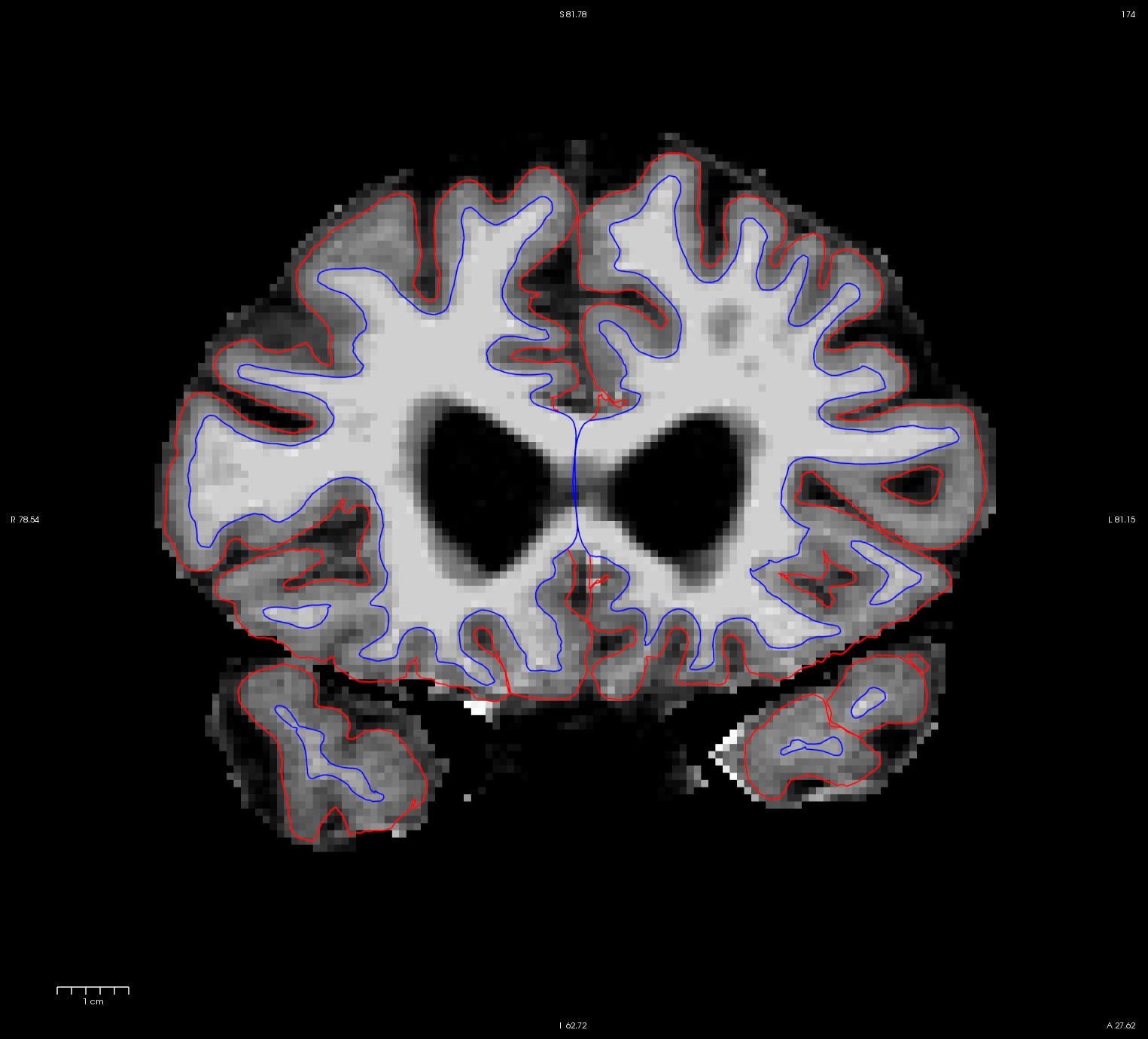
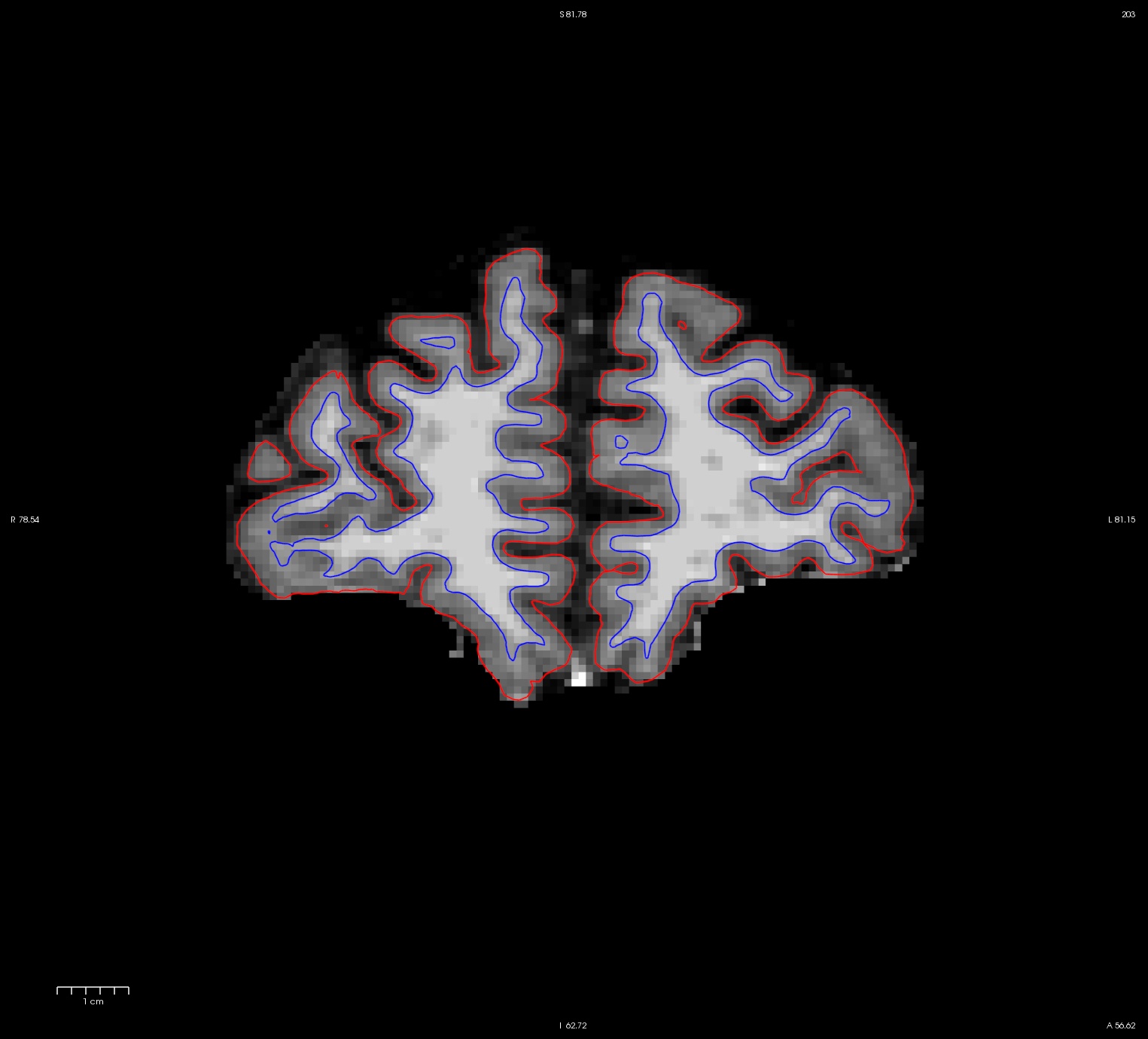
Compare the output volumes of the long (time point MR1) with the before-edit versions:

freeview -v OAS2_0057_MR1.long.OAS2_0057/mri/T1.mgz \
            OAS2_0057_MR1.long.OAS2_0057/mri/brainmask.mgz \
         -f OAS2_0057_MR1.long.OAS2_0057/surf/lh.pial:edgecolor=red \
            OAS2_0057_MR1.long.OAS2_0057/surf/rh.pial:edgecolor=red \
            OAS2_0057_MR1.long.OAS2_0057/surf/lh.white:edgecolor=blue \
            OAS2_0057_MR1.long.OAS2_0057/surf/rh.white:edgecolor=blue

freeview -v OAS2_0057_MR1.long.OAS2_0057_fixed/mri/T1.mgz \
            OAS2_0057_MR1.long.OAS2_0057_fixed/mri/brainmask.mgz \
         -f OAS2_0057_MR1.long.OAS2_0057_fixed/surf/lh.pial:edgecolor=red \
            OAS2_0057_MR1.long.OAS2_0057_fixed/surf/rh.pial:edgecolor=red \
            OAS2_0057_MR1.long.OAS2_0057_fixed/surf/lh.white:edgecolor=blue \
            OAS2_0057_MR1.long.OAS2_0057_fixed/surf/rh.white:edgecolor=blue

Here is the before image (left) of OAS2_0057_MR1.long.OAS2_0057 (slice 174) and the corresponding after image (right - slice 174).

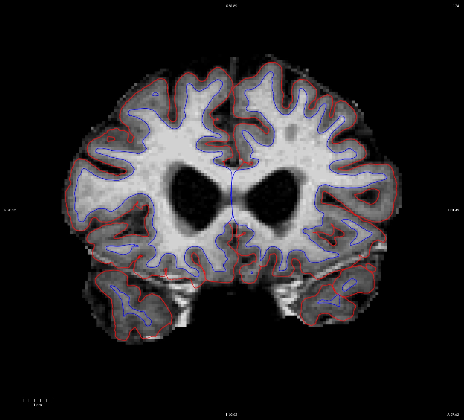
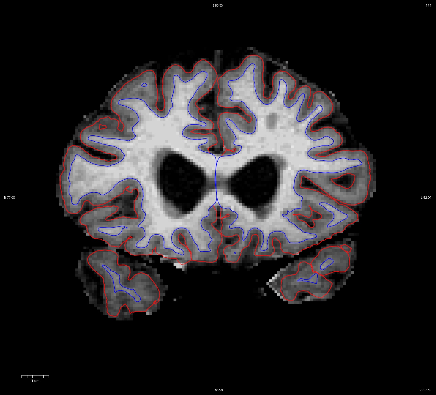
The same improvement should have occurred in OAS2_0057_MR2.long.OAS2_0057.

7. Control Points Edits

Sometimes, there are areas in the white matter with intensity lower than 110 and where the wm is not included in the surfaces. The best way to fix this problem is to add control points.

Take a look at the next subject, OAS2_0121 in all cross, base, and long to see if you can find the places that need control points. NOTE: We suggest only opening one freeview window at a time if you are using an old computer or one without much RAM. Freeview uses a large amount of memory, and may slow down your computer.

freeview -v OAS2_0121_MR1/mri/T1.mgz \
            OAS2_0121_MR1/mri/brainmask.mgz \
         -f OAS2_0121_MR1/surf/lh.pial:edgecolor=red \
            OAS2_0121_MR1/surf/rh.pial:edgecolor=red \
            OAS2_0121_MR1/surf/lh.white:edgecolor=blue \
            OAS2_0121_MR1/surf/rh.white:edgecolor=blue

freeview -v OAS2_0121_MR2/mri/T1.mgz \
            OAS2_0121_MR2/mri/brainmask.mgz \
         -f OAS2_0121_MR2/surf/lh.pial:edgecolor=red \
            OAS2_0121_MR2/surf/rh.pial:edgecolor=red \
            OAS2_0121_MR2/surf/lh.white:edgecolor=blue \
            OAS2_0121_MR2/surf/rh.white:edgecolor=blue

freeview -v OAS2_0121/mri/T1.mgz \
            OAS2_0121/mri/brainmask.mgz \
         -f OAS2_0121/surf/lh.pial:edgecolor=red \
            OAS2_0121/surf/rh.pial:edgecolor=red \
            OAS2_0121/surf/lh.white:edgecolor=blue \
            OAS2_0121/surf/rh.white:edgecolor=blue

freeview -v OAS2_0121_MR1.long.OAS2_0121/mri/T1.mgz \
            OAS2_0121_MR1.long.OAS2_0121/mri/brainmask.mgz \
         -f OAS2_0121_MR1.long.OAS2_0121/surf/lh.pial:edgecolor=red \
            OAS2_0121_MR1.long.OAS2_0121/surf/rh.pial:edgecolor=red \
            OAS2_0121_MR1.long.OAS2_0121/surf/lh.white:edgecolor=blue \
            OAS2_0121_MR1.long.OAS2_0121/surf/rh.white:edgecolor=blue

freeview -v OAS2_0121_MR2.long.OAS2_0121/mri/T1.mgz \
            OAS2_0121_MR2.long.OAS2_0121/mri/brainmask.mgz \
         -f OAS2_0121_MR2.long.OAS2_0121/surf/lh.pial:edgecolor=red \
            OAS2_0121_MR2.long.OAS2_0121/surf/rh.pial:edgecolor=red \
            OAS2_0121_MR2.long.OAS2_0121/surf/lh.white:edgecolor=blue \
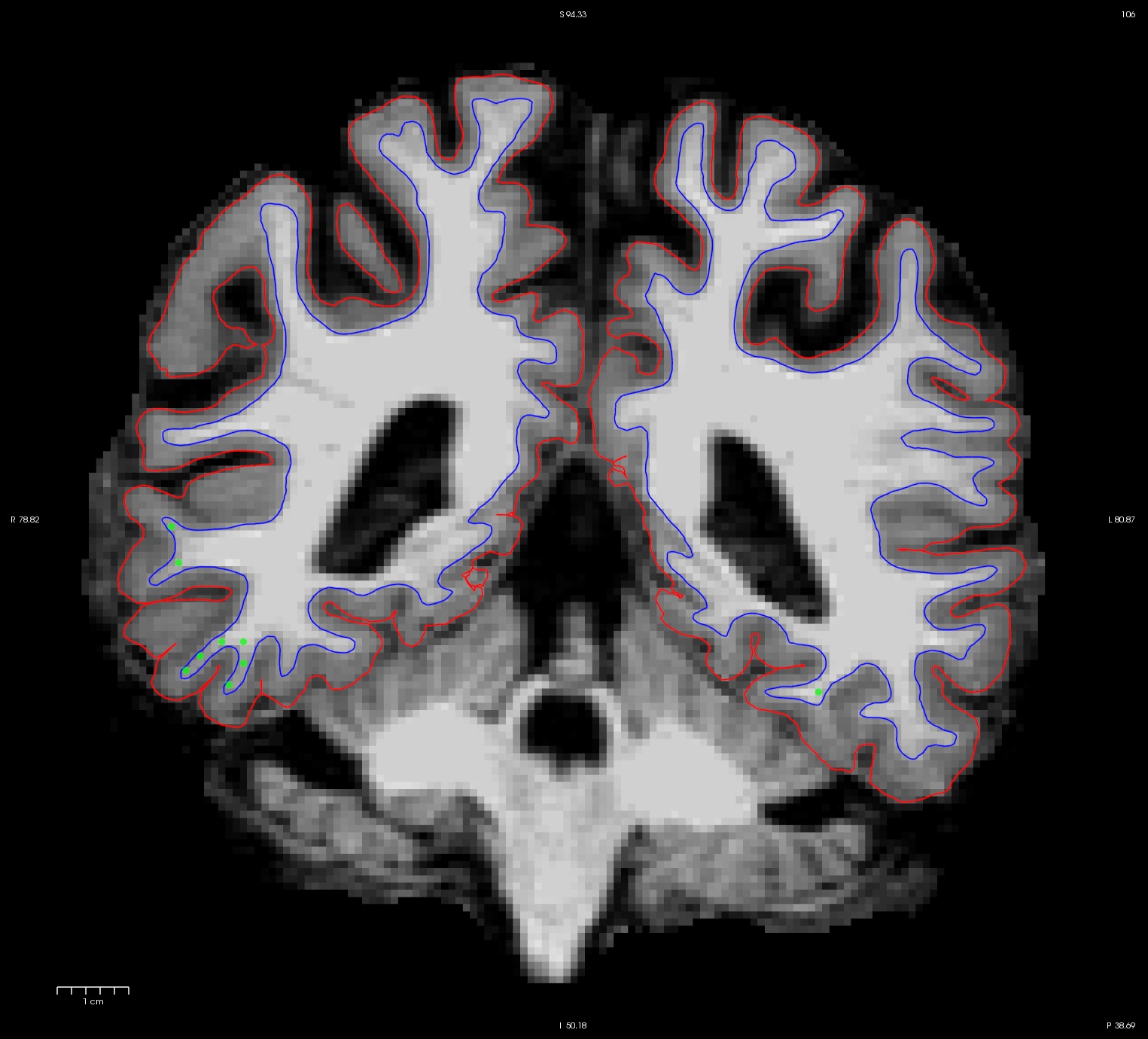
            OAS2_0121_MR2.long.OAS2_0121/surf/rh.white:edgecolor=blue

Notice that the intensity for the area in the bottom corner of the right hemisphere around slice 90 is only around 90 something instead of 110, and the surfaces here do not include all of the gm and wm. Because this problem occurs in both cross-sectionals, the base and subsequently the longitudinals are also affected. In cases like this, it depends on which data you are planning to use, you can choose to edit either the cross, base, or long. Control points work in all three stages.

In this example, we're demonstrating what the effect will be when adding control points at the very beginning of the stream - in the cross-sectionals. Find all the slices that have this problem and add control points carefully on the wm voxels.

7.1. Fixing the cross

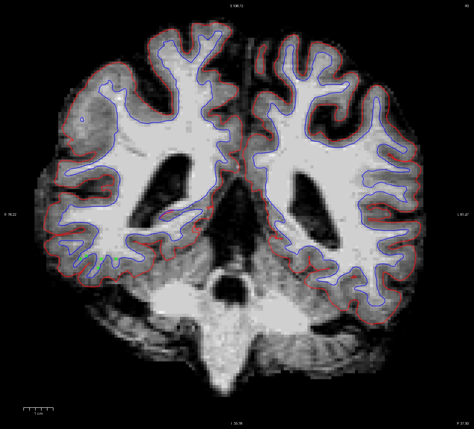
You want to add control points at the stem of white matter strands where voxel values are below 110. You can also add control points along the strand. Here is what we did. For cross sectional time point 1 (OAS2_0121_MR1), here is an example of coronal slice 90 before (left) and after (right) control points were added and the cross sectional was re-run.

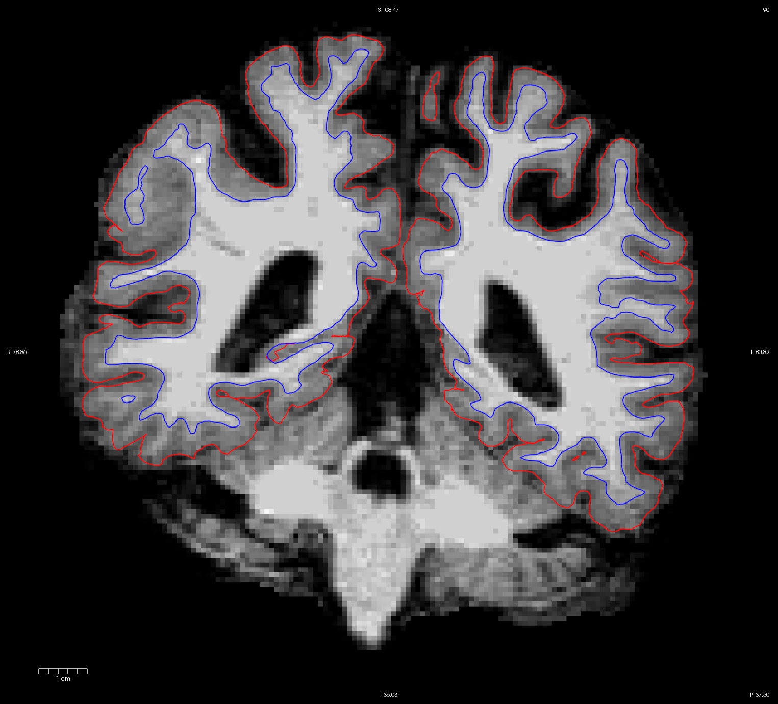
For cross time point 2 (OAS2_0121_MR2), here is an example of coronal slice 92 before and after control points are added

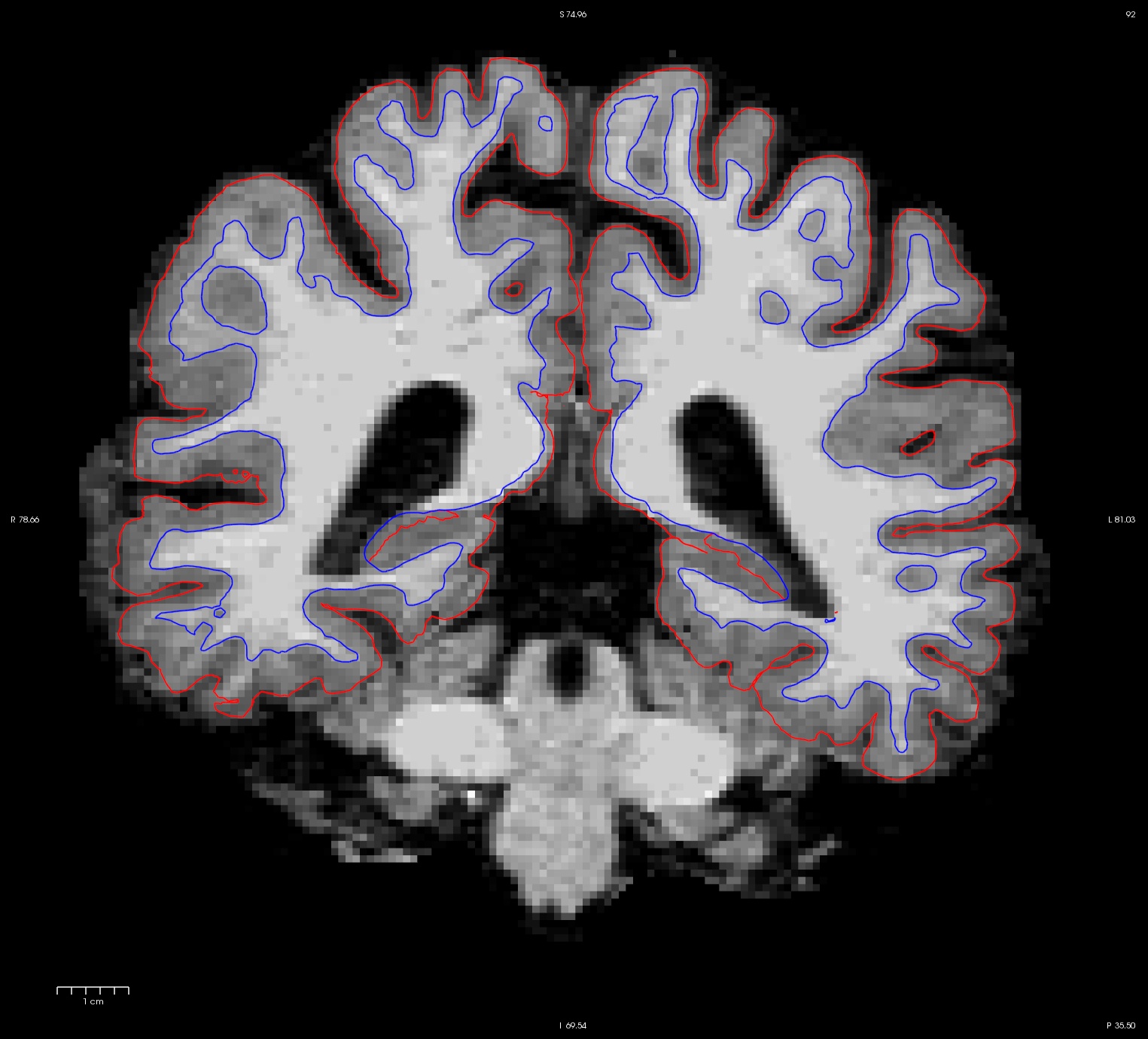
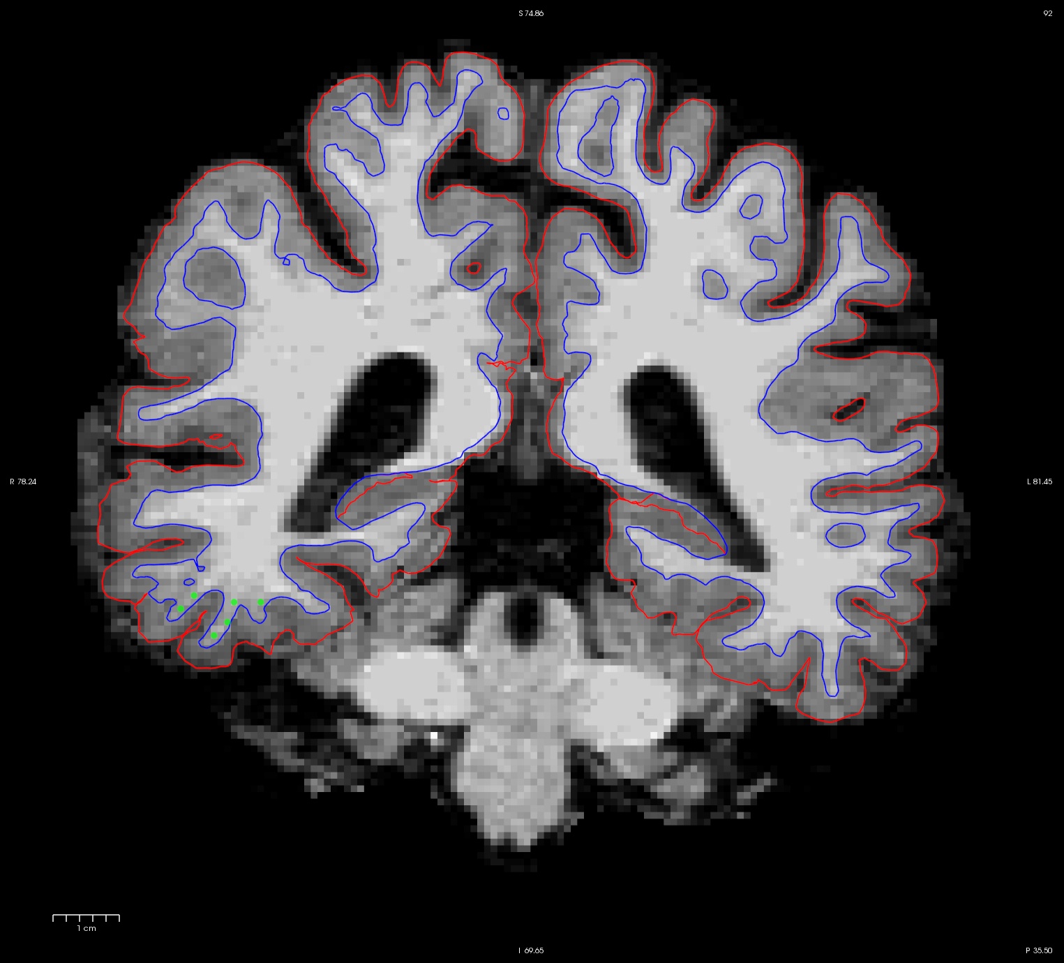
Once you are satisfied with your control points placements, save it, and run the following commands to complete the fixed cross sectional runs:

recon-all -subjid OAS2_0121_MR1 -autorecon2 -autorecon3

recon-all -subjid OAS2_0121_MR2 -autorecon2 -autorecon3

After that is complete (or when the CA normalization step is complete - you can check in the recon-all-status.log), you can start rerunning the base (remember to delete or rename the base if it already existed, e.g. mv OAS2_0121 OAS2_0121_old). Or, if you prefer, you can wait until the recons are complete to check whether you are satisfied with the results before beginning the next step.

To inspect the fixed version of these two timepoints, run:

freeview -v OAS2_0121_MR1_fixed/mri/T1.mgz \
            OAS2_0121_MR1_fixed/mri/brainmask.mgz \
         -f OAS2_0121_MR1_fixed/surf/lh.pial:edgecolor=red \
            OAS2_0121_MR1_fixed/surf/rh.pial:edgecolor=red \
            OAS2_0121_MR1_fixed/surf/lh.white:edgecolor=blue \
            OAS2_0121_MR1_fixed/surf/rh.white:edgecolor=blue

freeview -v OAS2_0121_MR2_fixed/mri/T1.mgz \
            OAS2_0121_MR2_fixed/mri/brainmask.mgz \
         -f OAS2_0121_MR2_fixed/surf/lh.pial:edgecolor=red \
            OAS2_0121_MR2_fixed/surf/rh.pial:edgecolor=red \
            OAS2_0121_MR2_fixed/surf/lh.white:edgecolor=blue \
            OAS2_0121_MR2_fixed/surf/rh.white:edgecolor=blue

7.2. Fixing/Rerunning the base

To rerun the base, you would run this command:

recon-all -base OAS2_0121 -tp OAS2_0121_MR1 -tp OAS2_0121_MR2 -all

Once you are done with the base, check to see whether the surfaces are now including all white matter (we ran the above command for you, results are in OAS2_0121_intermediate):

freeview -v OAS2_0121_intermediate/mri/T1.mgz \
            OAS2_0121_intermediate/mri/brainmask.mgz \
         -f OAS2_0121_intermediate/surf/lh.pial:edgecolor=red \
            OAS2_0121_intermediate/surf/rh.pial:edgecolor=red \
            OAS2_0121_intermediate/surf/lh.white:edgecolor=blue \
            OAS2_0121_intermediate/surf/rh.white:edgecolor=blue

Notice that although the surfaces improved, it is not perfect. In this case, you can add more control points to the base and would rerun with the command below (you would re-run the edited base without the _intermediate suffix as that is just a intermediate copy that we created for you):

recon-all -base OAS2_0121 -autorecon2 -autorecon3

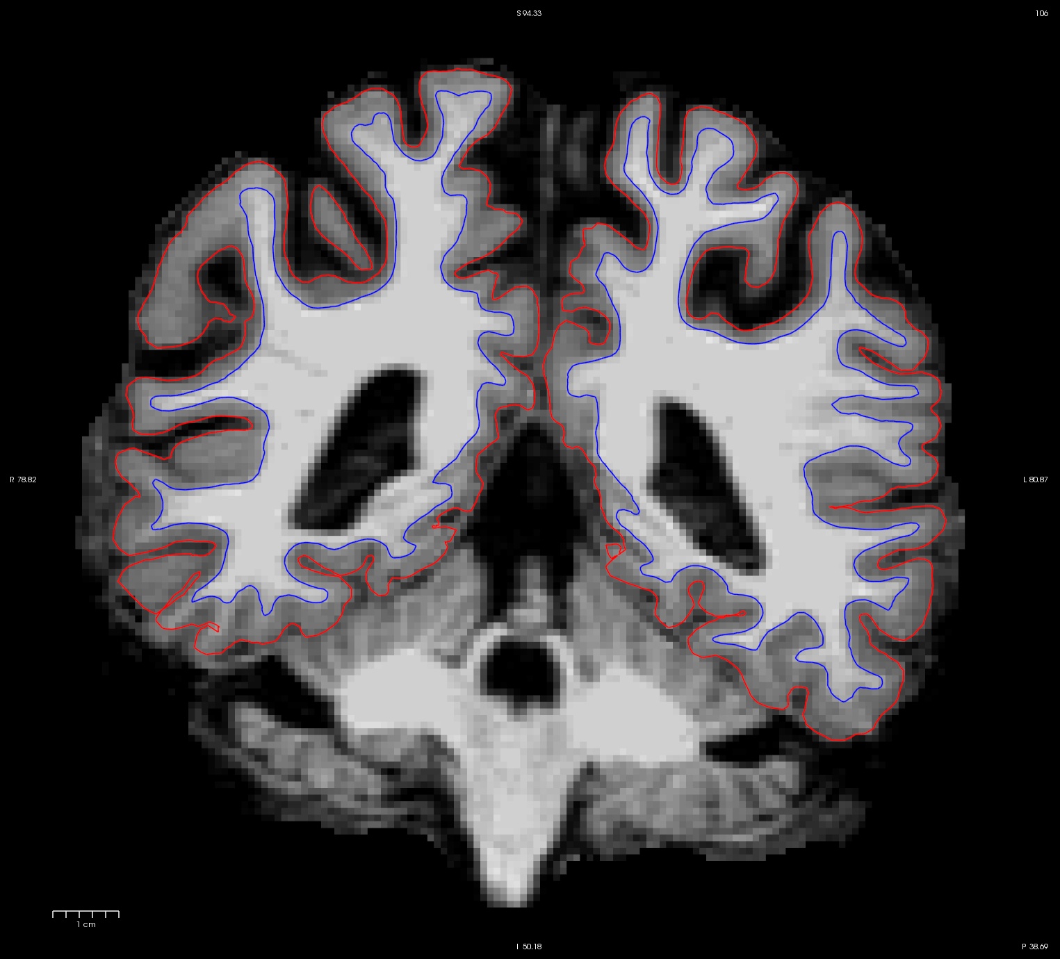
Now the base is much better. Compare these images at slice 106. These are taken from OAS2_0121_intermediate before more control points were added (below left) and OAS2_0121_fixed (below right). You can open these two volumes using Freeview, and also compare to the original base (OAS2_0121) before the cross sectionals were fixed if you want.

7.3. Rerunning the long

The last step is to rerun the longitudinals (also remember to remove/rename existing longitudinal directories first), which would be done with these commands:

recon-all -long OAS2_0121_MR1 OAS2_0121 -all

recon-all -long OAS2_0121_MR2 OAS2_0121 -all

---

Compare the output below

freeview -v OAS2_0121_MR1.long.OAS2_0121/mri/T1.mgz \
            OAS2_0121_MR1.long.OAS2_0121/mri/brainmask.mgz \
         -f OAS2_0121_MR1.long.OAS2_0121/surf/lh.pial:edgecolor=red \
            OAS2_0121_MR1.long.OAS2_0121/surf/rh.pial:edgecolor=red \
            OAS2_0121_MR1.long.OAS2_0121/surf/lh.white:edgecolor=blue \
            OAS2_0121_MR1.long.OAS2_0121/surf/rh.white:edgecolor=blue

freeview -v OAS2_0121_MR1.long.OAS2_0121_fixed/mri/T1.mgz \
            OAS2_0121_MR1.long.OAS2_0121_fixed/mri/brainmask.mgz \
         -f OAS2_0121_MR1.long.OAS2_0121_fixed/surf/lh.pial:edgecolor=red \
            OAS2_0121_MR1.long.OAS2_0121_fixed/surf/rh.pial:edgecolor=red \
            OAS2_0121_MR1.long.OAS2_0121_fixed/surf/lh.white:edgecolor=blue \
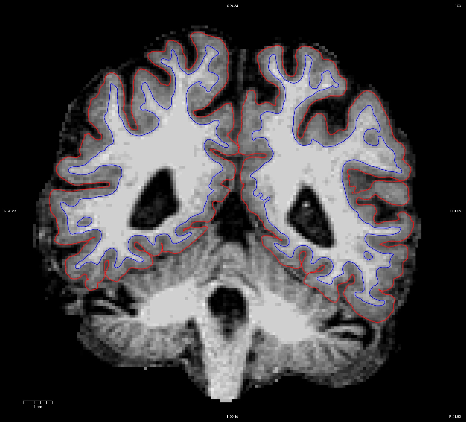
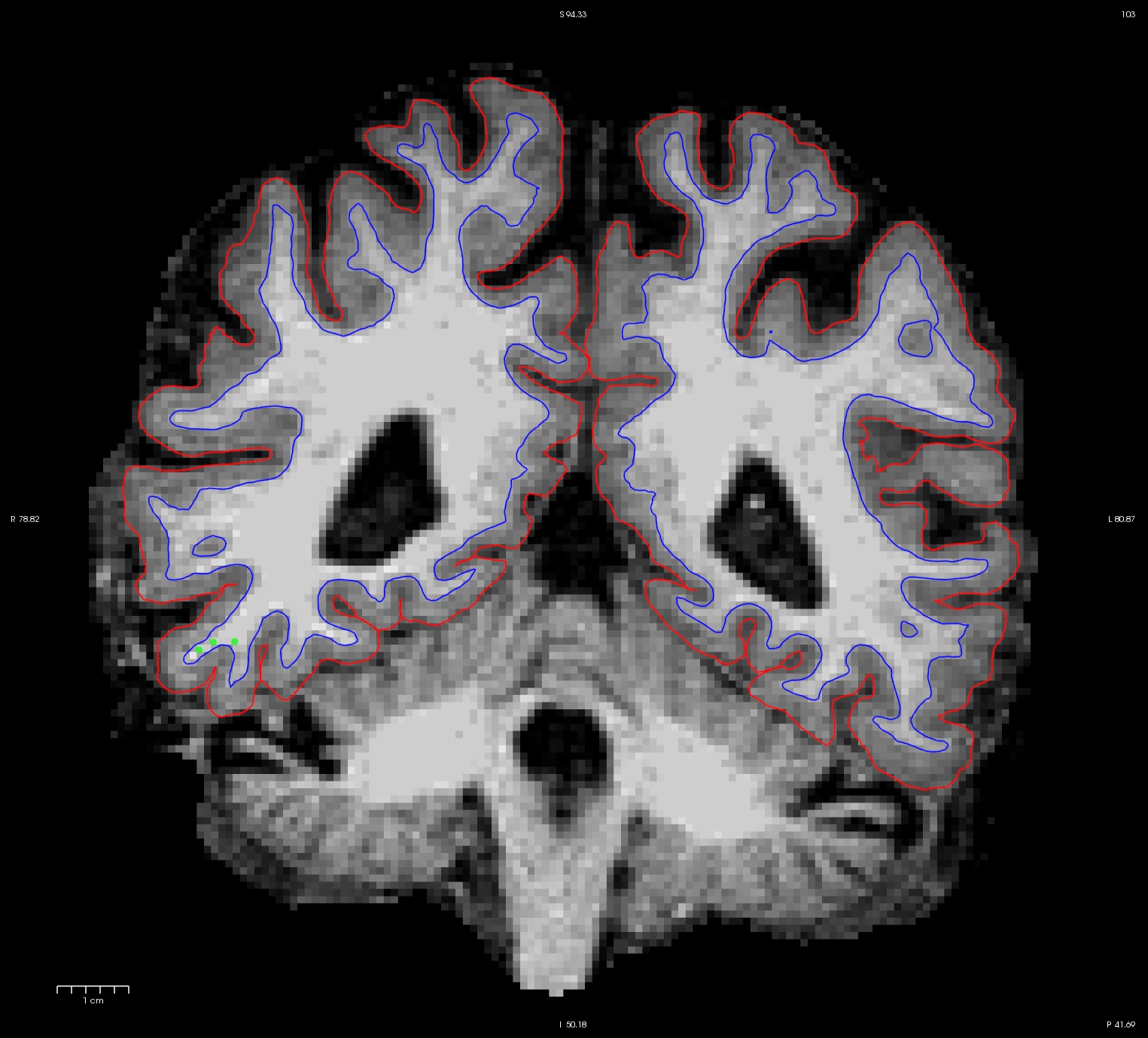
            OAS2_0121_MR1.long.OAS2_0121_fixed/surf/rh.white:edgecolor=blue

For the longitudinals, control points were automatically copied over from the cross-sectionals, and the surfaces were initialized from the base, therefore making a great improvement on the surfaces at this end of the stream.

The before (left) and after (right) images from OAS2_0121_MR1.long.OAS2_0121 at slice 107.

8. White Matter Edits

White matter edits are possibly the most common type of edits you will come across in data. In many cases, even a difference of 1 wm voxel can cause a huge defect in the surfaces. Take a look at the following subject. For this one, we will open the brainmask.mgz volume and compare it to the wm.mgz volume instead of T1.mgz. If you're using tkmedit instead of Freeview, load wm.mgz as your "Aux Volume". NOTE: We suggest only opening one freeview window at a time if you are using an old computer or one without much RAM. Freeview uses a large amount of memory, and may slow down your computer.

freeview -v OAS2_0185/mri/wm.mgz \
            OAS2_0185/mri/brainmask.mgz \
         -f OAS2_0185/surf/lh.pial:edgecolor=red \
            OAS2_0185/surf/rh.pial:edgecolor=red \
            OAS2_0185/surf/lh.white:edgecolor=blue \
            OAS2_0185/surf/rh.white:edgecolor=blue

freeview -v OAS2_0185_MR1/mri/wm.mgz \
            OAS2_0185_MR1/mri/brainmask.mgz \
         -f OAS2_0185_MR1/surf/lh.pial:edgecolor=red \
            OAS2_0185_MR1/surf/rh.pial:edgecolor=red \
            OAS2_0185_MR1/surf/lh.white:edgecolor=blue \
            OAS2_0185_MR1/surf/rh.white:edgecolor=blue

freeview -v OAS2_0185_MR2/mri/wm.mgz \
            OAS2_0185_MR2/mri/brainmask.mgz \
         -f OAS2_0185_MR2/surf/lh.pial:edgecolor=red \
            OAS2_0185_MR2/surf/rh.pial:edgecolor=red \
            OAS2_0185_MR2/surf/lh.white:edgecolor=blue \
            OAS2_0185_MR2/surf/rh.white:edgecolor=blue

freeview -v OAS2_0185_MR1.long.OAS2_0185/mri/wm.mgz \
            OAS2_0185_MR1.long.OAS2_0185/mri/brainmask.mgz \
         -f OAS2_0185_MR1.long.OAS2_0185/surf/lh.pial:edgecolor=red \
            OAS2_0185_MR1.long.OAS2_0185/surf/rh.pial:edgecolor=red \
            OAS2_0185_MR1.long.OAS2_0185/surf/lh.white:edgecolor=blue \
            OAS2_0185_MR1.long.OAS2_0185/surf/rh.white:edgecolor=blue

freeview -v OAS2_0185_MR2.long.OAS2_0185/mri/wm.mgz \
            OAS2_0185_MR2.long.OAS2_0185/mri/brainmask.mgz \
         -f OAS2_0185_MR2.long.OAS2_0185/surf/lh.pial:edgecolor=red \
            OAS2_0185_MR2.long.OAS2_0185/surf/rh.pial:edgecolor=red \
            OAS2_0185_MR2.long.OAS2_0185/surf/lh.white:edgecolor=blue \
            OAS2_0185_MR2.long.OAS2_0185/surf/rh.white:edgecolor=blue

Toggle between the two volumes (use the opacity slider) and see if you can spot an area where a simple wm edit will make a huge difference to the surfaces.

8.1. Making white matter edits

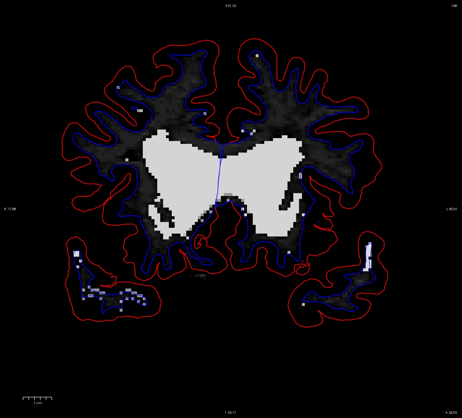
For the longitudinal stream, it is recommended that you make wm.mgz edits to the base. This is because even though the long transfers manual wm edits from the cross, it still takes the surfaces from the base, and if the base surfaces did not improve, neither will the long. The only way to make corrections to the base surfaces themselves is to edit wm.mgz on the base. Therefore, making wm.mgz edits right on the base can save you a lot of time. Of course it is best to edit all stages (all cross time points and base), but often it is sufficient to edit only the base. Were you able to find the area that needs intervention? Here is what we found. You can see below on the brainmask.mgz (left) that the pial surface is cutting through the wm. If you toggle to the wm.mgz, you can see that there are a few wm voxels missing.

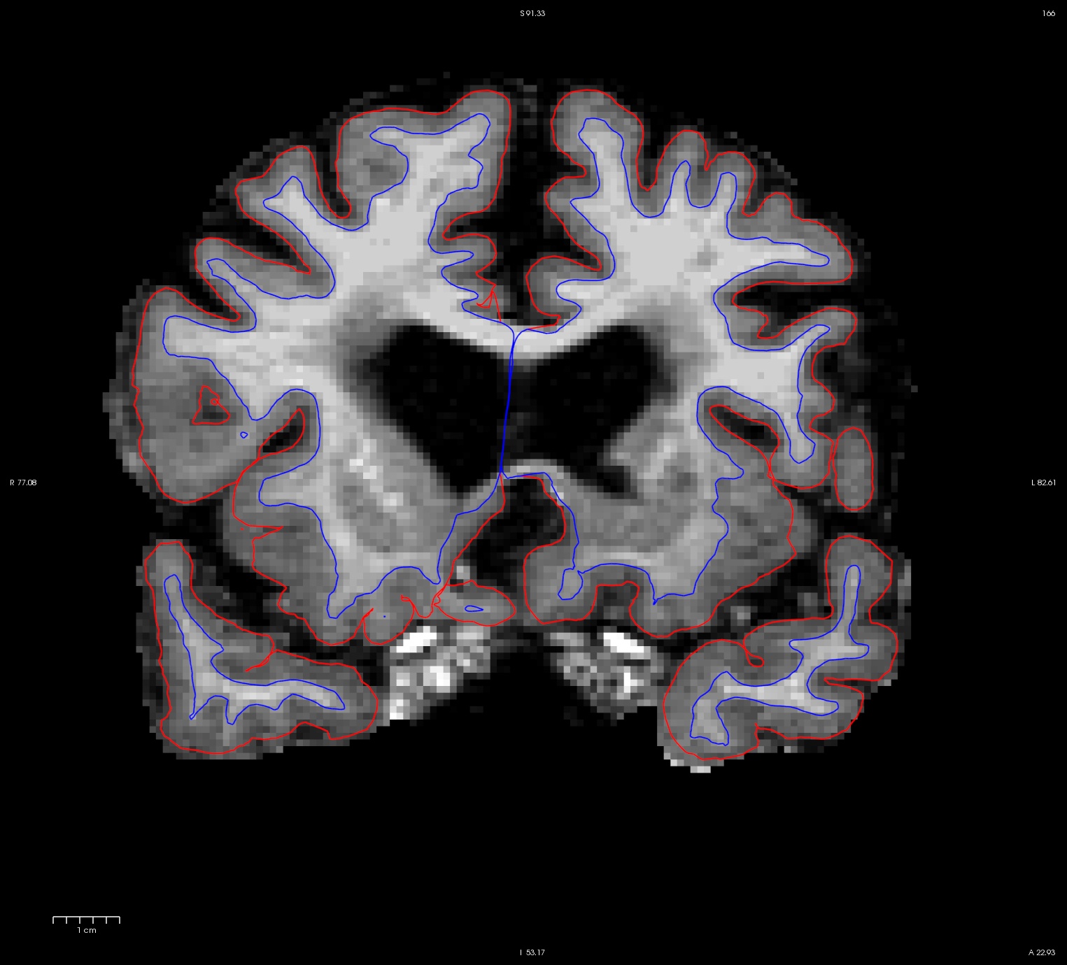
This happens at the tip of the lh temporal lobe within several slices. Below is an example of coronal slice 166.

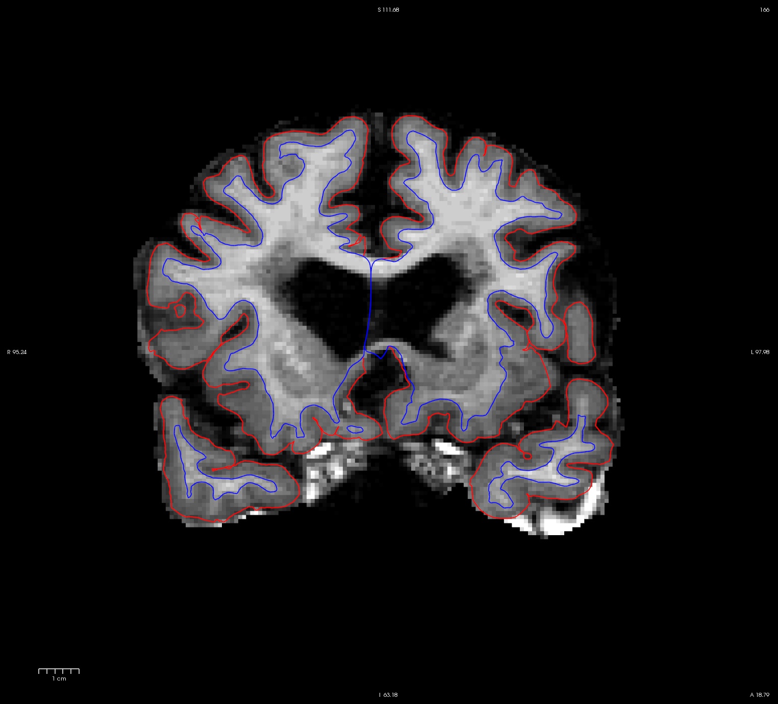
Add wm voxels to connect the wm together in all the slices that need it. Here is an example of what we did in slice 168. Bright wm voxels in the temporal lobes have been manually added.

---

After you are satisfied with your edits, save the edited volume and rerun the base.

recon-all -base OAS2_0185 -autorecon2-wm -autorecon3

After that is done, check the surfaces on base using Freeview (or tkmedit for older version of Freeview).

freeview -v OAS2_0185_fixed/mri/wm.mgz \
            OAS2_0185_fixed/mri/brainmask.mgz \
         -f OAS2_0185_fixed/surf/lh.pial:edgecolor=red \
            OAS2_0185_fixed/surf/rh.pial:edgecolor=red \
            OAS2_0185_fixed/surf/lh.white:edgecolor=blue \
            OAS2_0185_fixed/surf/rh.white:edgecolor=blue

This is what it should look like now in slice 166.

When the surfaces are all corrected, you would recreate the long (make sure you remove the long directories before the rerun - or at the very least, remove the wm.mgz files in all the mri sub-directories of the long runs).

recon-all -long OAS2_0185_MR1 OAS2_0185 -all

recon-all -long OAS2_0185_MR2 OAS2_0185 -all

---

Inspect your output:

freeview -v OAS2_0185_MR1.long.OAS2_0185_fixed/mri/wm.mgz \
            OAS2_0185_MR1.long.OAS2_0185_fixed/mri/brainmask.mgz \
         -f OAS2_0185_MR1.long.OAS2_0185_fixed/surf/lh.pial:edgecolor=red \
            OAS2_0185_MR1.long.OAS2_0185_fixed/surf/rh.pial:edgecolor=red \
            OAS2_0185_MR1.long.OAS2_0185_fixed/surf/lh.white:edgecolor=blue \
            OAS2_0185_MR1.long.OAS2_0185_fixed/surf/rh.white:edgecolor=blue

freeview -v OAS2_0185_MR2.long.OAS2_0185_fixed/mri/wm.mgz \
            OAS2_0185_MR2.long.OAS2_0185_fixed/mri/brainmask.mgz \
         -f OAS2_0185_MR2.long.OAS2_0185_fixed/surf/lh.pial:edgecolor=red \
            OAS2_0185_MR2.long.OAS2_0185_fixed/surf/rh.pial:edgecolor=red \
            OAS2_0185_MR2.long.OAS2_0185_fixed/surf/lh.white:edgecolor=blue \
            OAS2_0185_MR2.long.OAS2_0185_fixed/surf/rh.white:edgecolor=blue

See here that the improved surfaces in the base also correct the surfaces in the long. Compare MR1.long slice 166 in the before (left) and after (right) images below.

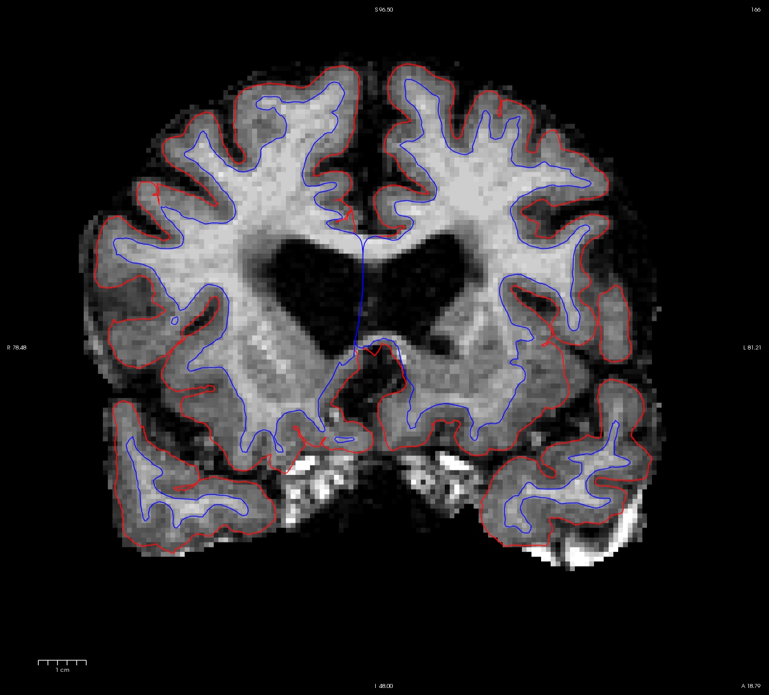
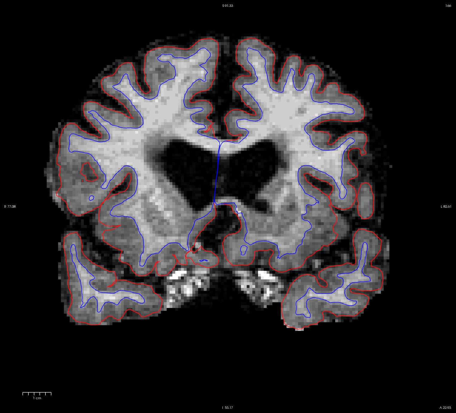
The same improvement should have occurred with MR2.longitudinal run.

---

MartinReuter

---

9. Quiz

You can test your knowledge of this tutorial by clicking here for a quiz!

---

Back to list of all tutorials
Back to course page