FreeSurfer Tutorial: Surface Group Analysis with Qdec
If you are taking one of the formally organized courses, the tutorial data is already installed on the computer provided to you. If not, then to follow this exercise exactly be sure you've downloaded the tutorial data set before you begin. If you choose not to download the data set you can follow these instructions on your own data, but you will have to substitute your own specific paths and subject names. If you are using the tutorial data please set the environmental variable TUTORIAL_DATA to the location to which you have downloaded the data (on the course laptops, it happens to be in /media/disk).
In this tutorial, you will learn how to perform statistical analysis of group surface-based data, including:
Preprocessing the group data
Constructing a qdec.table.dat file of subject demographics
Using Qdec to design and execute your analysis
- Interacting with the Qdec display
- Creating Regions of Interest (ROIs) for further analysis and a final check of your data
Assuming that all 'recon-all -all' processing has been completed for all subjects in the study, FreeSurfer's Qdec application can be used to perform inter-subject/group averaging and inference on the cortical surface. Qdec permits statistical inferences to be made about effects of interest in relation to error variance. The mri_glmfit command is used to model the data as a linear combination of effects related to variables of interest, confounds and errors. Qdec also allows for certain permutation testing and other means for correcting for multiple comparisons. For group analysis, this technique fits a general linear model (GLM) at each surface vertex to explain the data from all subjects in the study. In this section, a brief overview of linear modeling is presented and can be skipped if this material is already familiar. Other software packages have similar types of programs (e.g., FSL's GFEAT). Note that Qdec wraps the mri_glmfit utility, which has more extensive GLM capabilities than QDEC, but is a command-line-only tool. It has its own tutorial.
Introduction
Qdec
Qdec is a single-binary application included in the FreeSurfer distribution. QDEC is an acronym for Query, Design, Estimate, Contrast. It is intended to aid researchers in performing inter-subject / group averaging and inference on the morphometry data (cortical surface and volume) produced by the FreeSurfer processing stream. Qdec is a GUI front-end to a 'statistics engine' (the mri_glmfit binary, included in FreeSurfer, currently fills this role) intended to:
- select the subjects meeting the criteria under study
- generate the necessary input to the stats engine, which, for mri_glmfit, includes:
a Design matrix (called X in the GLM equation) containing the explanatory variables,
a parameter Estimate matrix (called A in the GLM equation), and
the Contrast vector(s)
- generate and optionally display the output data and/or images
Linear Modeling overview
Linear modeling describes the observed data as a linear combination of explanatory factors plus noise, and determines how well that description explains the data being analyzed. In order to understand how to perform group analysis in FreeSurfer, you need to understand the general linear model (GLM) and how to construct a GLM in matrix notation. You can click here for a review of this material. The notation we use here is:y=X*beta, where y is the vector observed data (e.g., thicknesses for each subject at a vertex), X is the known design matrix (e.g., gender, age), and beta is the vector of unknown parameter estimates (PEs). The interpretation of the PEs will depend upon how X is constructed. For example, they could be interpreted as a slope indicating the change of thickness with age. The analysis/estimation is then the process of computing beta given the data y and the design matrix X. A Null Hypothesis (H0) is constructed with a contrast matrix C. Inferences are drawn by testing whether the value gamma=Cb is zero.
Preprocess Group Data
set SUBJECTS_DIR
If you are using the tutorial data you will need to set your SUBJECTS_DIR to the directory with the group analysis data in it:
setenv SUBJECTS_DIR $TUTORIAL_DATA/buckner_data/tutorial_subjs/group_analysis_tutorial
cd $SUBJECTS_DIR
* this will set your SUBJECTS_DIR to the location where your tutorial data is located (the directory containing the group analysis subjects, assuming you have defined the variable TUTORIAL_DATA as indicated at the top of this tutorial). If you are not using the tutorial data you should set your SUBJECTS_DIR to the directory in which the subjects you will use for this tutorial are located. For the organized course, TUTORIAL_DATA is set for you.
recon-all
Prior to using the qdec application, your group subject data must be processed by the standard FreeSurfer processing stream, via the recon-all script. A freesurfer tutorial is available. This processing stream supplies the surfaces and morphometry data on each subject. The data in the tutorial set has been processed for you.
pre-smoothed fsaverage surfaces
Qdec needs each subject to have pre-computed smoothed data for the target surface (fsaverage is the default) for each measure (thickness, sulc, area, curv, etc.). Your SUBJECTS_DIR should contain either a link or a copy of the 'fsaverage' subject found in your $FREESURFER_HOME/subjects directory. Presmoothing the data onto the target surface is not part of the normal recon processing stream, but you can easily create this data with recon-all, using the command:
recon-all -s <subjid> -qcache
For the purposes of this tutorial, the -qcache command has been run for all of the subjects. The -qcache flag will run numerous back-to-back mris_preproc processes on your machine, so be prepared for it to run for about an hour. The help text of recon-all -help contains a section on other -qcache otpions.
qdec.table.dat
The primary input to Qdec is a text file, named qdec.table.dat, containing the subject IDs, and discrete and continuous factors, in table format. This is essentially a table of demographics for your subject including all the variables and factors that you wish to consider. Here is an example file:
fsid            gender  age diagnosis   Left-Cerebral-White-Matter
011121_vc8048   Female  70  Demented    202291
021121_62313-2  Female  71  Demented    210188
010607_vc7017   Female  73  Nondemented 170653
021121_vc10557  Male    75  Demented    142029
020718_62545    Male    76  Demented    186087
020322_vc8817   Male    77  Nondemented 149810
For each discrete factor, there should exist a file named <factor>.levels which lists all possible levels. For example, accompanying the example qdec.table.dat file must be a file named 'gender.levels' containing these lines:
Female
Male
and there must be a file named 'diagnosis.levels' containing these lines:
Demented
Nondemented
Of course you may have different discrete factor names and levels (or even no discrete factors, in which case all column data are assumed to be continous factors). Continuous factors do not need a <factor>.levels file to define them.
For organizational purposes it is best to make a directory called qdec within your $SUBJECTS_DIR. You can save the qdec.table.dat and <factor>.levels files in there. When Qdec runs it will also save your analyses to this directory. A qdec subdirectory, with a qdec.table.dat has been made for you. Here is a sample of what that looks like:
fsid  gender  age   Left-Hippocampus Right-Hippocampus
140   Female  18    4214             4190
049   Male    19    4543             4153
141   Female  20    3896             3741
084   Male    21    4804             4722
021   Male    22    4021             3969
093   Female  22    3603             3597
This file contains 40 subject IDs, their gender, age, left hippocampus volume, and right hippocampus volume. To accompany this file you will need to create a <factor>.levels text file to define the discrete factor names. You can do this using the text editor of your choice (emacs, vi, pico...). For this tutorial, the qdec.table.dat file already exists for you.
Optionally, your qdec.table.dat file can explicitly specify the SUBJECTS_DIR, by including it in the first non-commented line:
# This is a comment-line in the qdec.table.dat file.
# This explicitly specifies the SUBJECTS_DIR:
SUBJECTS_DIR /my/path/to/subject/data

.
.
.
fsaverage
For display purposes, you will need to have an average subject included in your SUBJECTS_DIR. !Freesurfer's fsaverage, made in MNI305 space, will do fine:
cd $SUBJECTS_DIR
if (! -e fsaverage) ln -s $FREESURFER_HOME/subjects/fsaverage
This will add a copy of fsaverage into your SUBJECTS_DIR.
For the purposes of this tutorial, fsaverage has already been linked to your $SUBJECTS_DIR.
If you wish to make your own average subject from your set you can do so using make_average_subject.
Usage
To start qdec, from your $SUBJECTS_DIR, simply type qdec:
setenv SUBJECTS_DIR $TUTORIAL_DATA/buckner_data/tutorial_subjs/group_analysis_tutorial
cd $SUBJECTS_DIR

qdec &
It may take a few seconds for Qdec to open. The ampersand directs the terminal to run this process in the background, so you may see your command prompt return before Qdec opens.
Subjects
When Qdec opens you are looking at the Subjects tab. The first thing you will need to do is to load your qdec.table.dat file. Click File -> Load Data Table, or you can use the  button, and traverse to your subjects directory and select the qdec.table.dat file. When you click Open, it should load the file, the contents scrolling-by in the terminal window. If the data is loaded correctly, you should see in the terminal window a summary, like this example:
.
.
.
1  gender  discrete 2
    1  Female
    2  Male
2  age  continuous 0
3  Left-Hippocampus  continuous 0
4  Right-Hippocampus  continuous 0
                Continuous Factors:         Mean:       StdDev:
                -------------------         -----       -------
                                age        57.175        26.940
                   Left-Hippocampus      3645.850       579.214
                  Right-Hippocampus      3725.325       555.961

Number of subjects:   40
Number of factors:    4 (1 discrete, 3 continuous)
Number of classes:    2
Number of regressors: 8
The factors (gender, age, Left-Hippocampus, and Right-Hippocampus) should appear in a list under 'Data Table View' on the control panel. If you choose a factor from this list a scatter plot of your data will appear in the window. Choose 'age', and the display should like this:
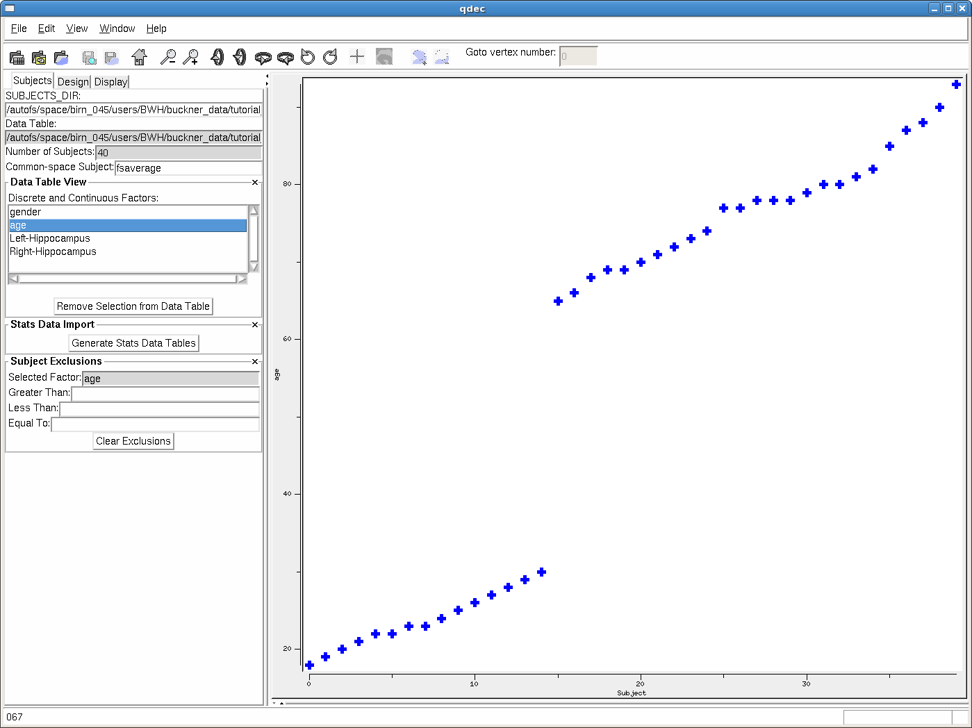
The x-axis has the subject number (taken from the order the subjects are listed in the qdec.table.dat), and the y-axis has the value of the variable you've selected. In the example shown you can see a plot of the ages of all 40 subjects. You can use this to visually check your data for outliers. In Qdec if you roll your cursor over one of the points on the plot you can find out which subject it is, the ID will be shown in the lower left corner of the Qdec interface.
Stats Data Import
It is possible to import the aseg and aparc data from the FreeSurfer-processed group data. To do so, press the 'Generate Stats Data Tables' button. This will run the FreeSurfer utilities asegstats2table and aparcstats2table on your group data. Upon completion (you should see the progress in the terminal screen), then the 'Generate Stats Data Tables' button becomes a menu-selection list. Within that menu, you can select 'aseg.volume'. Upon doing so, the volumetric data for various subcortical structures are displayed. You could choose for example 'Left-Lateral-Ventricle', then click 'Add Selection to Data Table'. Upon doing so, it will appear in the 'Discrete and Continuous Factors' display of the 'Data Table View'. 'Left-Lateral-Ventricle' is now available as a possible factor in your analysis ('Left-Hippocampus' and 'Right-Hippocampus' were imported from aseg.volume in this manner). If you select 'Left-Lateral-Ventricle' in the 'Data Table View', then the volumetric data for all the subjects is plotted. You can look for patterns or outliers. If you suspect an outlier, right-click on that point in the scatter-plot. You can then either exclude that subject, or examine it in tkmedit or tksurfer, to check for possible problems in the original scan data. Lastly, you can save this newly imported data (in this case, 'Left-Lateral-Ventricle') to your qdec.table.dat file by selecting 'Save Data Table' from the File menu (but dont do this for the tutorial).
Design
When you click-over to the Design tab your discrete (gender) and continuous (age, Left-Hippocampus, Right-Hippocampus and Left-Lateral-Ventricle) factors should appear.
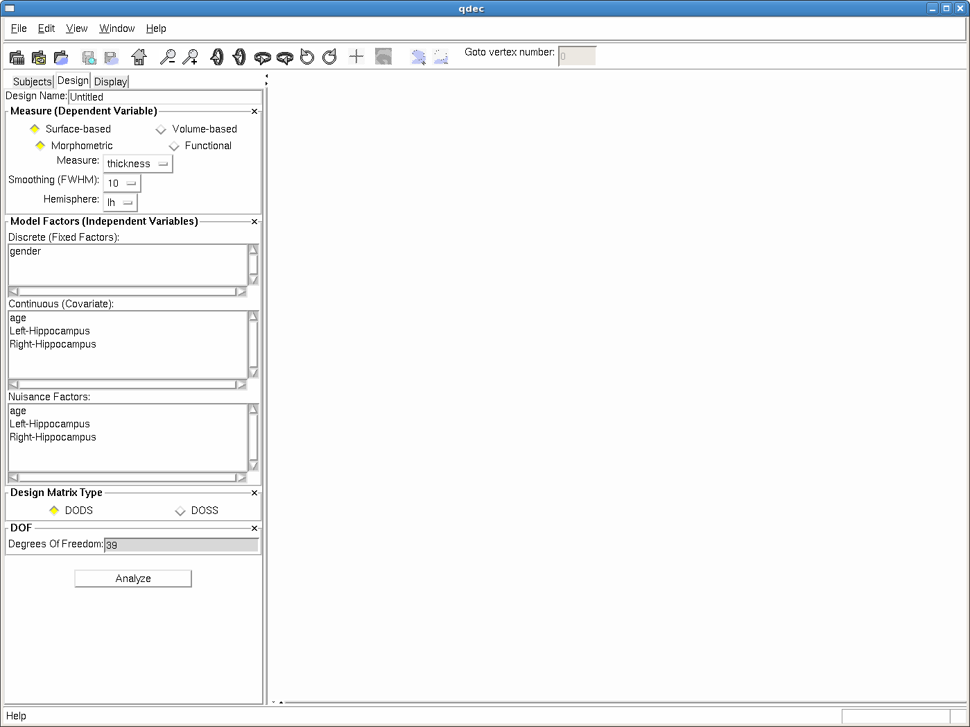
You can select up to four factors in the Design tab to regress against. For the tutorial data, you could select 'gender' and 'age' and 'Left-Hippocampus' and 'Right-Hippocampus', or any combination of those. Nuisance Factor menu in Design tab allows selection of any number of continuous variables of which will be treated as 'nuisance variables' in the glm (contrast matrix will have value '0' for these). For simplicity in this example, choose only 'age' in the Continuous variables menu, leaving the 'Measure', 'Hemisphere' and 'Smoothing' at their defaults (thickness, lh and 10mm). Before you click the 'Analyze' button you will want to name your Design, something like 'lh-thickness-age-fwhm10', and enter that into the "Design Name" text entry box at the top of the window. Now click the 'Analyze' button and the stats-engine will begin processing, executing the mri_glmfit executable. Upon clicking 'Analyze', the terminal will display the output of this processing. Also, progress information is shown in the bottom bar of the Qdec application. An analysis make take a minute or two.
Display
Once the analysis is complete (taking up to several minutes for a large subject set), you can click the Display tab and the fsaverage inflated surface will appear in the display window. You will see a list of questions summarizing the various analyses that were completed. 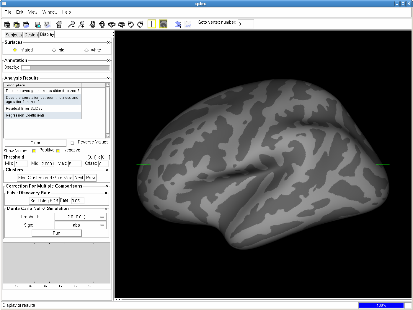
You can click on one of these questions to load the results. If you click on Does the correlation between thickness and age differ from zero it will display the statistically significant regions where age and thickness are correlated. Here is an example display:
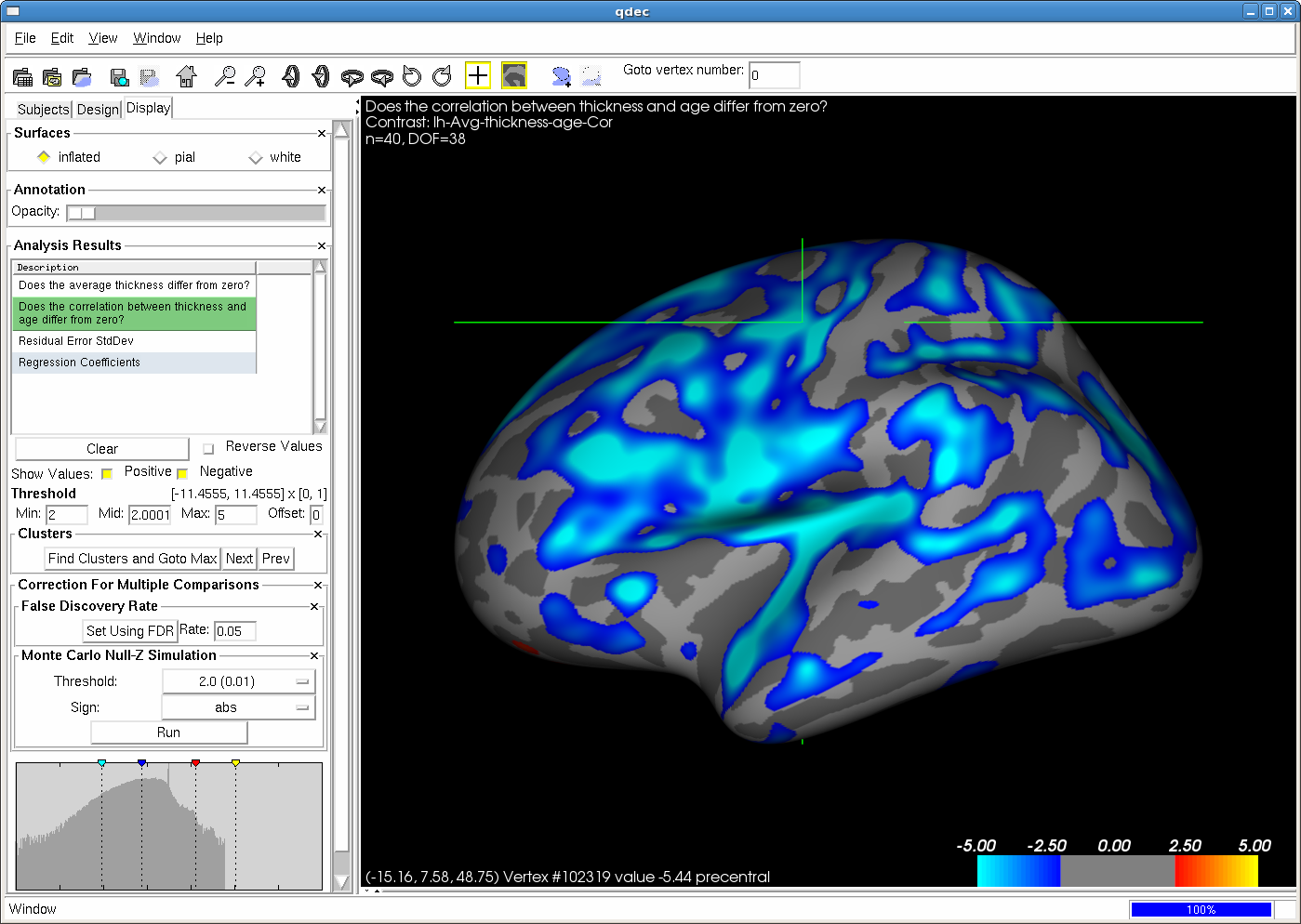
'FindClustersAndGotoMax' button runs mri_surfcluster on a selected result, which will find clusters based on currently selected display threshold, output a table of results to the terminal, and move the cursor to the max vertex in the #1 cluster. 'Next' and 'Prev' buttons allow cycling movement of the cursor through the found clusters. On the displayed image, notice the green cross-hairs that indicate the vertex you have currently selected. You can change vertices and display a plot of the data for a particular vertex by left-clicking on a point while holding-down the Ctrl key. If you'd like to turn off the cursor display you can use the  button. Here is an example plot that corresponds to the shown selected vertex:
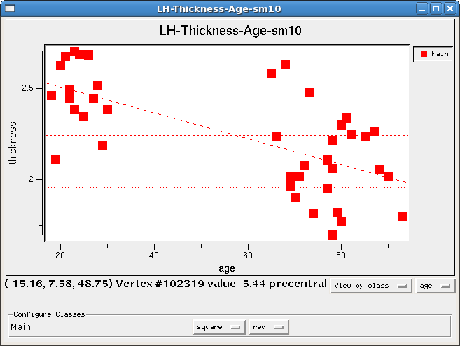
The plot shows your measure on the y-axis (vertical) - in this case, cortical thickness - and the variable on the x-axis (horizontal) - in this case, age. Each data point on the plot is representative of an individual subject, denoting their age and cortical thickness at the vertex you have selected. For this example at this vertex, we can see that the cortex is thinning with age. The information at the bottom of the both the plot window and the Qdec window shows that this vertex has surface coordinates (-15.16, 7.58, 48.75) and is Vertex# 102319. The significance value is -5.44 and it is in the precentral region. The significance in this display is a -log(10)p value, and not a straight p value.
In addition to this you can also do correction for multiple comparisons by Monte Carlo cluster-wise simulation making use of pre-run data, making run-time near instantaneous.
Interacting with your data
Rotating, Panning and Zoom You can rotate the display, hold-down the left mouse button and move the mouse. Holding-down the middle button while moving the mouse will move the display in the window. Holding-down the right mouse button while moving will zoom the display.
There are buttons at the top of the Qdec display that will rotate and zoom as well:
 - rotates up 90 degrees
 - rotates down 90 degrees
 - rotates right 90 degrees
 - rotates left 90 degrees
 - rotates counterclockwise 90 degrees
 - rotates clockwise 90 degrees
 - zoom out
 - zoom in
If you get it rotated too far, the home button  will reset it.
Parcellation Display The cortical parcellation is loaded into Qdec upon opening. On the Display tab you can adjust the annotation opacity. There may be a slight delay while the display updates, be patient!
Sliding the button to the right will begin to show the parcellation annotation underneath the overlay. You can bring the opacity to a level that is useful in your interaction with the data. When you have selected a point, which is accomplished by holding down the ctrl key and left-clicking the mouse, the information at the bottom of the window will tell you what region, or parcellation unit, the point is found.
Significance Thresholds
You can also adjust the threshold levels for the overlay on the Display tab.
When setting a color scale, you're interested in two things: the threshold (i.e., the value below which the vertex will be transparent - Min), and the saturation point (i.e., the value beyond which the color will not change - Max). In Qdec you can also specify the point where the color will reach the midpoint, with Mid on the control panel (by default Mid is set to just higher than Min. The meaning of these thresholds depends upon the nature of the data you have loaded as the overlay. The map you are currently viewing is -log10(p), where p is the significance, so a Min of 2 will display all vertices with p<.01 and a Max of 5 will show vertices of p<.00001 as the same color. You can lower the threshold to 1.3, 2, 3, to show all vertices with p<.05. You could raise the threshold to 4, 5, 6 to show all vertices with p<.0001.
Variations on Design
With Qdec it is easy to design and run a variety of different analyses. For the first example we looked simply at age and thickness in our subjects. Click back to the Design tab and select gender, to add it to the design. You will want to change the name of the design, call it 'lh-thickness-age-gender-fwhm10', and click Analyze. When the analysis is done running, click the Display tab and see that there are additional questions in the list summarizing the various analyses that were completed. Among the questions displayed now are Does the Thickness--age correlation differ between male and female? and Does the average thickness differ between male and female? Click on one of these questions to display the statistically significant regions where the age and thickness correlation are different in men and women, or the average thickness is different in men and women (respectively). Similarly, you can add in one of the other continous variables - hippocampal volume - and run that design.
You can change your design even more, if you click back to the Design tab, you can change your measure from thickness to something else - area, area.pial, volume, sulc, curv, and jacobian_white are your choices. You can also change your level of smoothing - 0, 5, 10, 15, 20, and 25 are your choices. And you can perform any of these on the left (lh) or right (rh) hemispheres. Take a few minutes to select a new design to run, remember to call it something new before you hit Analyze so that the directory of results can be saved.
Define a Region of Interest
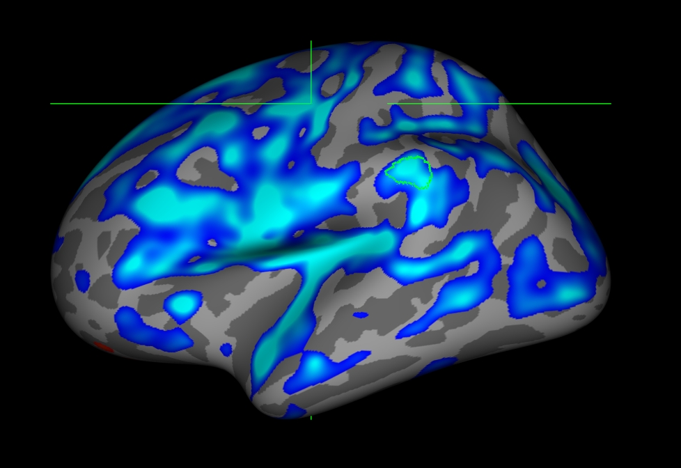
FreeSurfer has the ability to compute statistics averaged over a defined region of interest (ROI), which is another popular way to test statistical hypotheses and a good way to check your data. To define a label that marks a region of interest (ROI) on the surface hold down shift then left click and drag to draw your ROI. When drawing your ROI, draw slowly, allowing the display to catch up with you if necessary. There is no need to worry about closing the ROI precisely, when you are done and release the mouse button QDEC will automatically close the ROI for you. You should then see a green outline of the ROI you drew, like this:
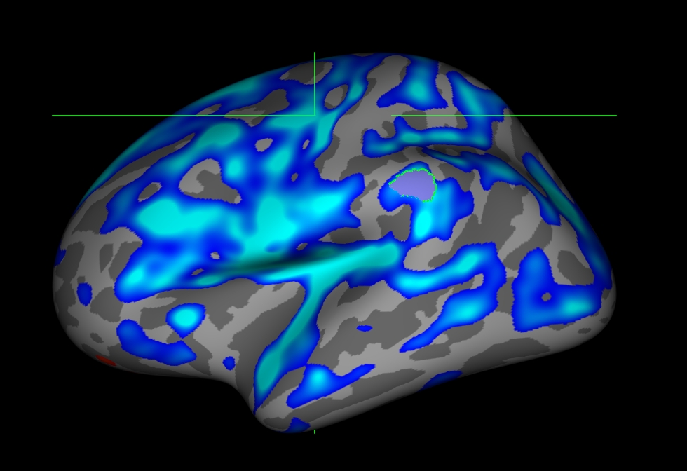
You can then select the add the selection to the ROI button  , and your label should now be filled in with purple, like this:
If you do not add your label to the ROI and you start to draw again, QDEC will erase your first label and begin a second. If you have added something to the ROI and want to remove it you can use the remove selection from ROI button  . When you are finished you can save your label by selecting File --> Save Label or clicking the
  save label button. A dialog box will pop up, and you can choose the location and name to save your label. For this example you can call your label lh.supramarg.label, since it is a label of the supramarginal gyrus, and click Save.
It may then be useful to map this label to all of the individual subjects in your group study, to either extract statistical values from this region or to visualize the area on each subject to check the integrity of your results. You can do this automatically by selecting File --> Map Label to Subjects..., a dialog box will pop up asking for the label name, you can enter everything before the .label of the name, so for this example enter lh.supramarg, and click Ok (OPTIONAL as it takes a few minutes for this to finish). This will use mri_label2label to map this label from your average surface onto all the subjects in your study. When it is complete (this can take several minutes) each subject will have a file named lh.supramarg.label in its label subdirectory. But for tutorial purposes, you can run the following command to map the label onto a subject.
mri_label2label --srclabel lh.supramarg --srcsubject fsaverage --trgsubject 004 --trglabel lh.supramarg --regmethod surface --hemi lh
The above command creates the label lh.supramarg.label in 004/label/ directory. This label can be loaded onto each subject's surface in tksurfer, or opened on the volume in tkmedit (not shown in this tutorial).
mris_anatomical_stats You can use mris_anatomical_stats to get a set of statistics on each individual label you've created. The command to run this on the label lh.supramarg.label that you generated for subject 004 is:
cd $SUBJECTS_DIR
mris_anatomical_stats -l lh.supramarg.label \
  -t lh.thickness -b -f 004/stats/lh.supramarg.stats 004 lh
This will output a stats file to 004/stats/lh.supramarg.stats, which looks like this. This file gives the number of vertices, surface area, gray matter volume, average thickness and st. deviation, mean curvature, gaussian curvature, folding index, and curvature index for this region only. You can run this same command on all your subjects to generate these statistics. You could then use aparcstats2table to generate one space delimited table of all these measures for your subjects.
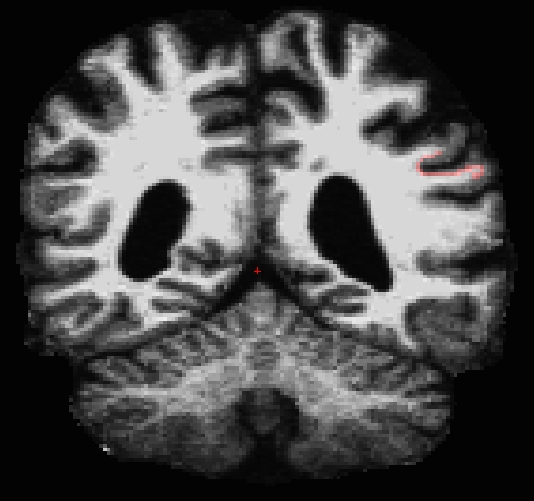
In addition, it might be a good idea to visualize this label on each subject, to be sure there is not a defect in the surface causing your result. You can look at your label in tkemdit on the volume with the command:
tkmedit 004 brainmask.mgz -label lh.supramarg.label
If you scroll towards the posterior end of the brain (coronal slice 80), you will find your label. Typically you would load the surfaces as well, but for this tutorial, it is easier to find the label without them.
Correction for Multiple-Comparisons
See this page for information on support for correction for multiple comparisons in Qdec. Note that it is not a tutorial. A more in-depth tutorial on this subject is found here.
Miscellaneous
Qdec supports some customizations via the .Qdecrc file.
(end of qdec tutorial)
