Anatomical ROI analysis
This tutorial gives a brief introduction to anatomical ROI analysis, including understanding FreeSurfer label files, extracting ROI measures from label files, and creating individual and group statistics files for further analyses.
1. Preparations
1.1. If You're at an Organized Course
If you are taking one of the formally organized courses, everything has been set up for you on the provided laptop. The only thing you will need to do is run the following commands in every new terminal window (aka shell) you open throughout this tutorial. Copy and paste the commands below to get started:
export SUBJECTS_DIR=$TUTORIAL_DATA/buckner_data/tutorial_subjs/group_analysis_tutorial
cd $SUBJECTS_DIR
To copy: Highlight the command in the box above, right click and select copy (or use keyboard shortcut Ctrl+c), then use the middle button of your mouse to click inside the terminal window to paste (or use the keyboard shortcut Ctrl+Shift+v).Press enter to run the command. These two commands set the SUBJECTS_DIR variable to the directory where the data is stored and then navigates into this directory. You can now skip ahead to the tutorial (below the gray line).
1.2. If You're not at an Organized Course
If you are NOT taking one of the formally organized courses, then to follow this exercise exactly be sure you've downloaded the tutorial data set before you begin. If you choose not to download the data set you can follow these instructions on your own data, but you will have to substitute your own specific paths and subject names. These are the commands that you need to run before getting started:
<source_freesurfer>
export TUTORIAL_DATA=<path_to_your_tutorial_data>
export SUBJECTS_DIR=$TUTORIAL_DATA/buckner_data/tutorial_subjs/group_analysis_tutorial
cd $SUBJECTS_DIR
If you are not using the tutorial data you should set your SUBJECTS_DIR to the directory in which the recon(s) of the subject(s) you will use for this tutorial are located.
2. Relationship between segmentation, parcellation and LookUp Table (LUT)
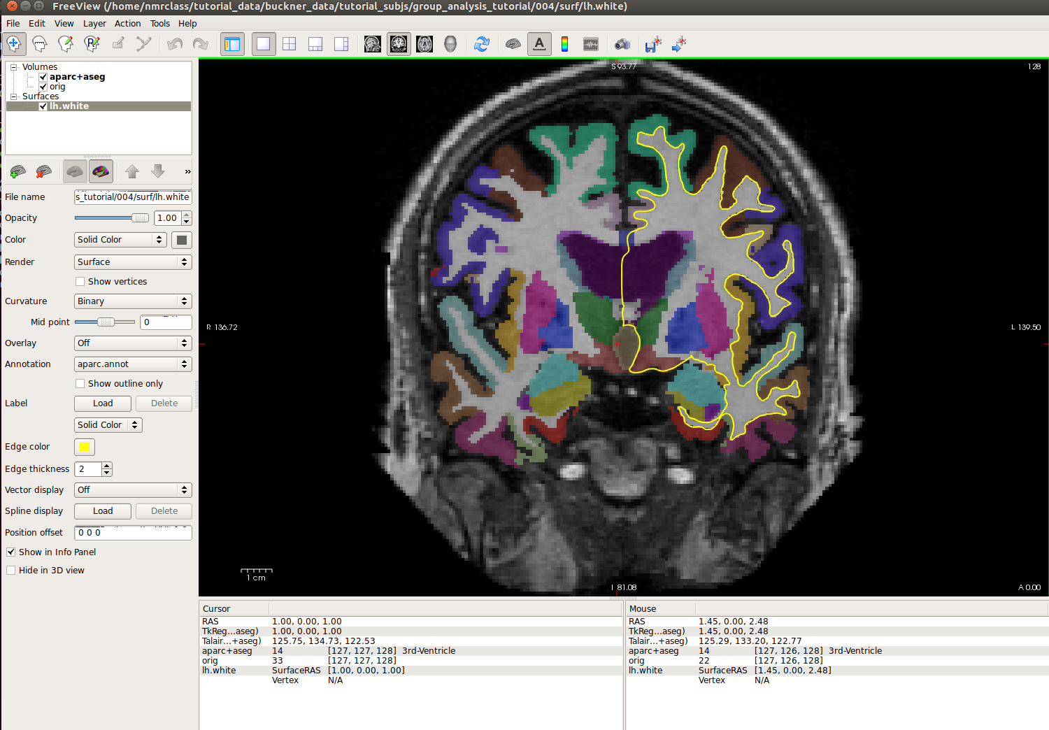
In this exercise, you will examine a segmentation, parcellation, and color lookup table to understand how they are related. Open the subject in Freeview using the following command and select 'coronal' view at the top menu bar:
freeview -v 004/mri/orig.mgz \
004/mri/aparc+aseg.mgz:colormap=lut:opacity=0.4 \
-f 004/surf/lh.white:annot=aparc.annot
NOTE: The backslash allows you to copy and paste multiple lines of code as one command. We use this throughout the tutorials to display the commands in a more easy-to-read manner, while still allowing you to copy and paste. Whenever you are typing in your own commands, instead of copying and pasting a command written out across multiple lines, a backslash is not necessary.
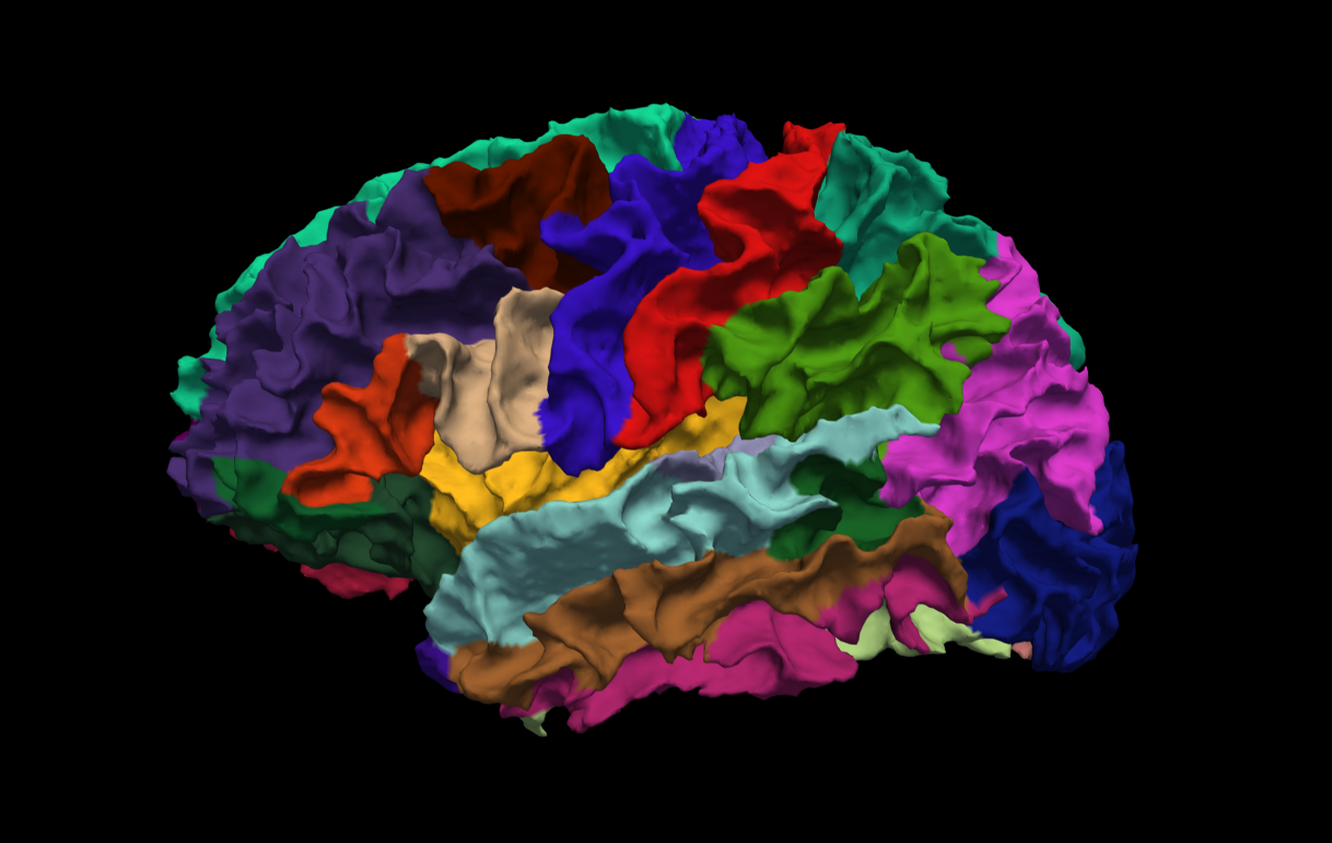
The above command opens the orig and aparc+aseg segmentation volume (aparc+aseg.mgz) as well as the cortical surface parcellation (aparc.annot) on the white surface in the left hemisphere. Note that the default parcellation uses the Desikan/Killiany atlas. There is also the option to use the Destrieux atlas parcellation, where the surface is parcellated into more anatomical regions than the Desikan/Killiany atlas.


Note: The aparc+aseg.mgz file shows the parcellated cortical ribbon at the same time as the segmented subcortical structures. The colormap=lut tells Freeview to display the aparc+aseg.mgz file with colors according to the look up table (LUT). The aparc+aseg.mgz uses the Desikan-Killiany atlas. To see the Destrieux atlas, you would load fsaverage/mri/aparc.a2009s+aseg.mgz Run the following commands in a new terminal window to display the contents of the LUT:
cd $FREESURFER_HOME
less FreeSurferColorLUT.txt
You can hit the 'Page Up' and 'Page Down' buttons on your keyboard to scroll through the text file. Or click here to view the contents of the file. (To exit the less command, hit 'q' on your keyboard.)
Things to do -- Navigating between freeview and the LUT:
- Choose the coronal view and click on a cortical structure in the brain.
- See the structure name next to 'aparc+aseg' in the Cursor section below the main viewing window. For example, it may say ctx-lh-precentral. Notice which hemisphere is specified.
- Look at the number listed immediately after the 'aparc+aseg'. For example, it may say 1024.
- Find that value in the LUT, which you have opened using the command mentioned above.
- Verify that it is the same structure you chose in freeview.
- Do the same with a subcortical structure of your choice.
You can close freeview once you are done. To get out of the less command, type 'q' for quit and hit enter.
3. Label files
To accurately map a manually drawn or pre-existing label of a region of interest to several subjects in your study, you should first register your label to or draw your label on fsaverage (a template to which all subjects run with FreeSurfer have been registered to) and then use the mri_label2label command to map the label to individual subjects. An example of the command you would use is illustrated below using the FreeSurfer-generated lh.BA45_exvivo.label (Brodmann area 45, part of Broca's area involved in language). Please run:
cd $SUBJECTS_DIR
mri_label2label \
  --srcsubject fsaverage \
  --srclabel $FREESURFER_HOME/subjects/fsaverage/label/lh.BA45_exvivo.label \
  --trgsubject 004 \
  --trglabel 004/label/lh.BA45_exvivo.label \
  --hemi lh \
  --regmethod surface
For more information about this command, type mri_label2label --help inside your terminal. Important flags:
- --srcsubject (the source subject)
- --srclabel (the input label file from source subject)
- --trgsubject (target subject you are mapping the label to)
- --trglabel (output label file on target subject)
- --regmethod (specify if you want the registration to occur on the surface or in the volume)
Our target subject in this example was 004. You can now view the label on this subject in Freeview. First load the subject:
freeview -v 004/mri/orig.mgz
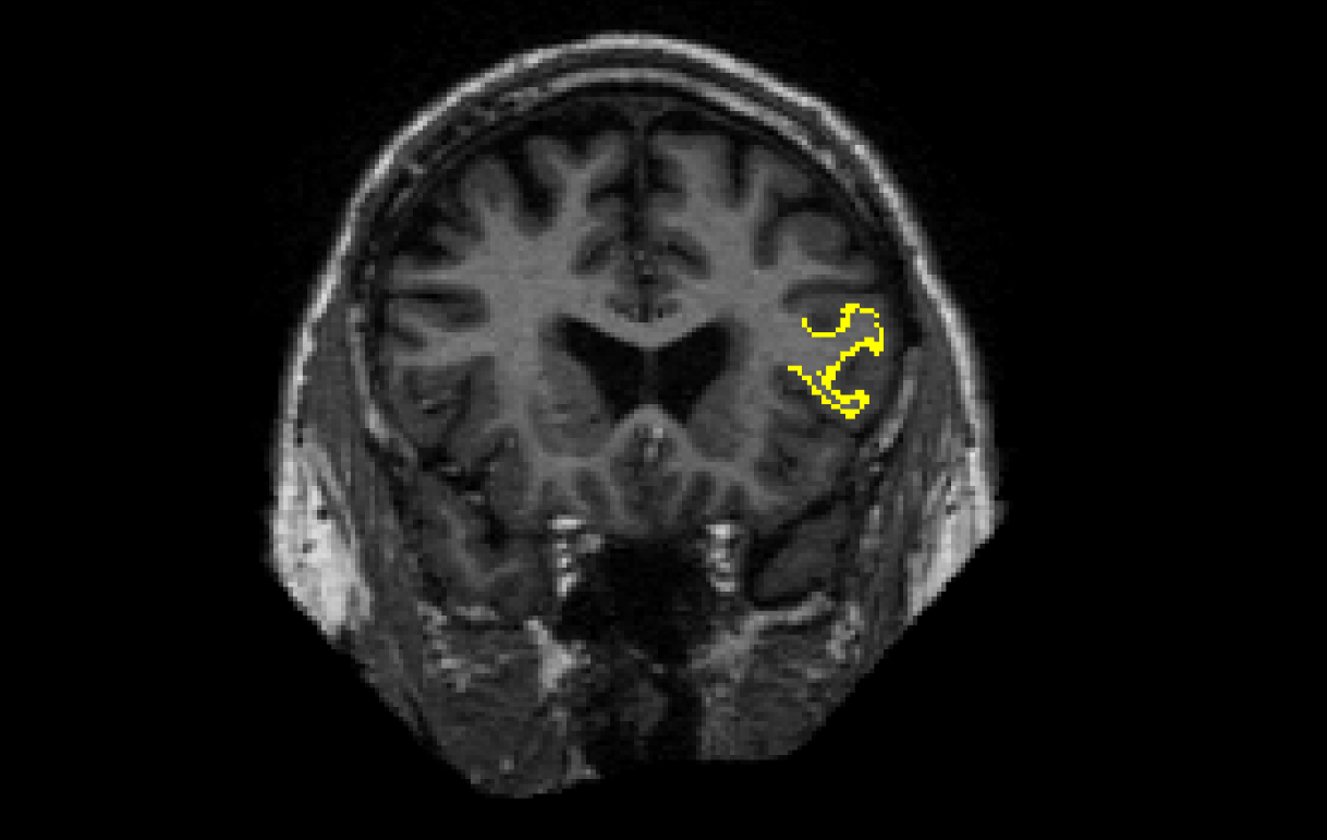
Then on the menu bar click File > Load ROI  choose lh.BA45_exvivo.label and hit 'Open'. The label is visible in coronal slices 130 through 178. For the purposes of this exercise, we will view the label in slice 153. To jump to that slice, double click on the coordinates [127,127,128] next to where it says 'orig' in the Cursor window pane. The last number is the slice number. Change it to 153 and hit enter.

To view the label on the surface, first load the subject's inflated surface in Freeview (in another terminal window) using the command below. At the top menu bar, select the 3D view.
freeview -f 004/surf/lh.inflated
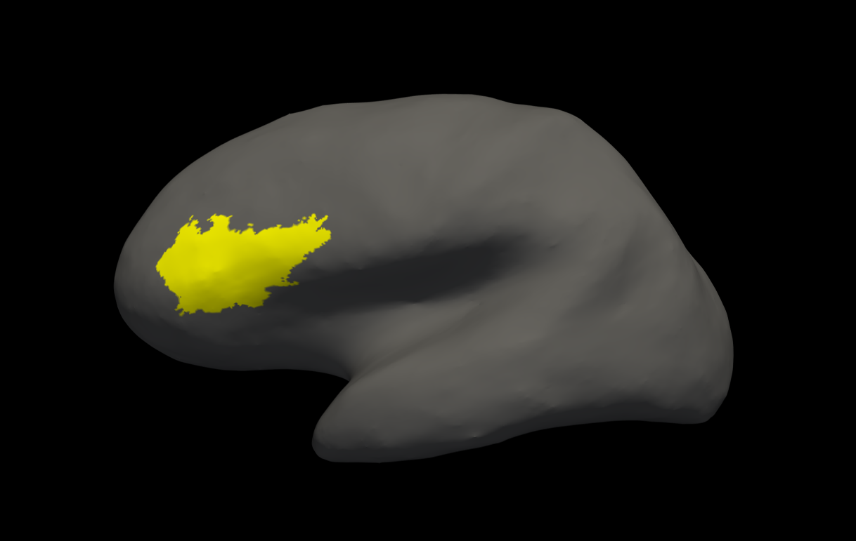
On the left menu, click on the drop down menu next to 'Curvature' and select 'Off'. Next to 'Label', select 'Load'. In the window that pops up, navigate to the label directory if it is not already in it and select lh.BA45_exvivo.label. Hit 'Open'. The label loaded on the inflated surface will look like this:

Note: If you want to use a pre-existing label and register it to fsaverage, be aware that this might involve two instances of resampling and the results might not be as accurate as they would be if you drew the label on fsaverage. Please contact the FreeSurfer team to get more details on this process if you have any concerns. You can close freeview once you are done.
4. Individual Stats files
During the FreeSurfer processing stream, via the recon-all script, some statistical output files are generated. They are kept in each subjects' stats/ subdirectory and are generated for the subcortical segmentation (aseg) and the cortical parcellation (aparc). These tables include information on each labeled region for the individual subject. You can view these output files via the terminal or a text editor.
4.1. aseg.stats
The statistical output from the subcortical segmentation, called aseg.stats, is a regular text file and will contain the volumes of specific structures. For example, you can obtain information such as the volume of left hippocampus and its mean intensity from this file.
cd $SUBJECTS_DIR/004/stats
less aseg.stats
At the head of the text file there will be information about the command that was run, the version used, the user who ran it and a time stamp. Following this there is information about the volume of the entire brain.
The next section of this file defines the column headers, field name, and units for the rest of the table. We can expect to see the Segmentation Id, Number of Voxels, Volume, Structure Name, Intensity normMean, Intensity normStdDev, Intensity normMin, Intensity normMax, and Intensity normRange for each entry in the table. The "norm" stats are extracted for each segmented structure from $SUBJECTS_DIR/004/mri/norm.mgz.
The remainder of the table shows this information for all the structures that are labeled in the aseg. (Remember, press 'q' if you want to quit the 'less' command).
As you may see below, the various headings don't line up perfectly in the terminal (or text editors). This is because the text file is formatted for spreadsheet programs.
# Title Segmentation Statistics
#
# generating_program mri_segstats
# cvs_version $Id: mri_segstats.c,v 1.121 2016/05/31 17:27:11 greve Exp $
# cmdline mri_segstats --seg mri/aseg.mgz --sum stats/aseg.stats --pv mri/norm.mgz --empty --brainmask mri/brainmask.mgz --brain-vol-from-seg --excludeid 0 --excl-ctxgmwm --supratent --subcortgray --in mri/norm.mgz --in-intensity-name norm --in-intensity-units MR --etiv --surf-wm-vol --surf-ctx-vol --totalgray --euler --ctab /space/freesurfer/build/pub-releases/v6.0.0/freesurfer/ASegStatsLUT.txt --subject 004
# sysname  Linux
# hostname compute-0-39
# machine  x86_64
# user     zkaufman
# anatomy_type volume
#
# SUBJECTS_DIR /autofs/cluster/freesurfer/subjects/test/buckner_data/stable6
# subjectname 004
# Measure BrainSeg, BrainSegVol, Brain Segmentation Volume, 1262276.000000, mm^3
# Measure BrainSegNotVent, BrainSegVolNotVent, Brain Segmentation Volume Without Ventricles, 1187271.000000, mm^3
# Measure BrainSegNotVentSurf, BrainSegVolNotVentSurf, Brain Segmentation Volume Without Ventricles from Surf, 1186951.705907, mm^3
# Measure VentricleChoroidVol, VentricleChoroidVol, Volume of ventricles and choroid plexus, 69043.000000, mm^3
# Measure lhCortex, lhCortexVol, Left hemisphere cortical gray matter volume, 259221.573235, mm^3
# Measure rhCortex, rhCortexVol, Right hemisphere cortical gray matter volume, 258713.044172, mm^3
# Measure Cortex, CortexVol, Total cortical gray matter volume, 517934.617407, mm^3
# Measure lhCerebralWhiteMatter, lhCerebralWhiteMatterVol, Left hemisphere cerebral white matter volume, 239218.899217, mm^3
# Measure rhCerebralWhiteMatter, rhCerebralWhiteMatterVol, Right hemisphere cerebral white matter volume, 236617.189283, mm^3
# Measure CerebralWhiteMatter, CerebralWhiteMatterVol, Total cerebral white matter volume, 475836.088500, mm^3
# Measure SubCortGray, SubCortGrayVol, Subcortical gray matter volume, 66911.000000, mm^3
# Measure TotalGray, TotalGrayVol, Total gray matter volume, 686541.617407, mm^3
# Measure SupraTentorial, SupraTentorialVol, Supratentorial volume, 1131346.705907, mm^3
# Measure SupraTentorialNotVent, SupraTentorialVolNotVent, Supratentorial volume, 1062303.705907, mm^3
# Measure SupraTentorialNotVentVox, SupraTentorialVolNotVentVox, Supratentorial volume voxel count, 1060851.000000, mm^3
# Measure Mask, MaskVol, Mask Volume, 1740098.000000, mm^3
# Measure BrainSegVol-to-eTIV, BrainSegVol-to-eTIV, Ratio of BrainSegVol to eTIV, 0.701763, unitless
# Measure MaskVol-to-eTIV, MaskVol-to-eTIV, Ratio of MaskVol to eTIV, 0.967408, unitless
# Measure lhSurfaceHoles, lhSurfaceHoles, Number of defect holes in lh surfaces prior to fixing, 70, unitless
# Measure rhSurfaceHoles, rhSurfaceHoles, Number of defect holes in rh surfaces prior to fixing, 59, unitless
# Measure SurfaceHoles, SurfaceHoles, Total number of defect holes in surfaces prior to fixing, 129, unitless
# Measure EstimatedTotalIntraCranialVol, eTIV, Estimated Total Intracranial Volume, 1798722.304401, mm^3
# SegVolFile mri/aseg.mgz
# SegVolFileTimeStamp  2017/01/19 21:37:44
# ColorTable /space/freesurfer/build/pub-releases/v6.0.0/freesurfer/ASegStatsLUT.txt
# ColorTableTimeStamp 2017/01/18 17:00:02
# InVolFile  mri/norm.mgz
# InVolFileTimeStamp  2017/01/19 04:08:57
# InVolFrame 0
# PVVolFile  mri/norm.mgz
# PVVolFileTimeStamp  2017/01/19 04:08:57
# Excluding Cortical Gray and White Matter
# ExcludeSegId 0 2 3 41 42
# VoxelVolume_mm3 1
# TableCol  1 ColHeader Index
# TableCol  1 FieldName Index
# TableCol  1 Units     NA
# TableCol  2 ColHeader SegId
# TableCol  2 FieldName Segmentation Id
# TableCol  2 Units     NA
# TableCol  3 ColHeader NVoxels
# TableCol  3 FieldName Number of Voxels
# TableCol  3 Units     unitless
# TableCol  4 ColHeader Volume_mm3
# TableCol  4 FieldName Volume
# TableCol  4 Units     mm^3
# TableCol  5 ColHeader StructName
# TableCol  5 FieldName Structure Name
# TableCol  5 Units     NA
# TableCol  6 ColHeader normMean
# TableCol  6 FieldName Intensity normMean
# TableCol  6 Units     MR
# TableCol  7 ColHeader normStdDev
# TableCol  7 FieldName Itensity normStdDev
# TableCol  7 Units     MR
# TableCol  8 ColHeader normMin
# TableCol  8 FieldName Intensity normMin
# TableCol  8 Units     MR
# TableCol  9 ColHeader normMax
# TableCol  9 FieldName Intensity normMax
# TableCol  9 Units     MR
# TableCol 10 ColHeader normRange
# TableCol 10 FieldName Intensity normRange
# TableCol 10 Units     MR
# NRows 45
# NTableCols 10
# ColHeaders  Index SegId NVoxels Volume_mm3 StructName normMean normStdDev normMin normMax normRange
  1   4     33163    33215.1  Left-Lateral-Ventricle            12.6416    10.9375     0.0000    77.0000    77.0000
  2   5      1200     1221.1  Left-Inf-Lat-Vent                 26.6925    14.4286     0.0000    75.0000    75.0000
  3   7     12677    13179.5  Left-Cerebellum-White-Matter      76.4266     8.8658    13.0000   106.0000    93.0000
  4   8     51530    51612.4  Left-Cerebellum-Cortex            49.6198    11.7537     0.0000   100.0000   100.0000
  5  10      7568     7259.4  Left-Thalamus-Proper              74.9564    13.4454     2.0000   126.0000   124.0000
  6  11      5505     5379.5  Left-Caudate                      64.2171    11.3418    30.0000   106.0000    76.0000
  7  12      7815     7535.4  Left-Putamen                      68.3104    10.7348    11.0000   104.0000    93.0000
-
-
-
4.2. aparc.stats
The statistical output from the cortical parcellation, called lh.aparc.stats and rh.aparc.stats, is a regular text file and will contain the thickness of specific structures. For example, you can obtain information such as, how big is left superior temporal gyrus and its average thickness from this file.
cd $SUBJECTS_DIR/004/stats
less lh.aparc.stats
This file takes the same format as the aseg.stats. The measures at the top show the number of vertices in the cortex (NumVert) and the surface area of the cortex (SurfArea). This part of the file also tells us that the lh.aparc.annot is being used as the annotation file (AnnotationFile ../label/lh.aparc.annot).
The next section of this file defines the column headers, field name, and units for the rest of the table. We can expect to see the Structure Name, Number of Vertices, Surface Area, Gray Matter Volume, Average Thickness, Thickness StDev, Integrated Rectified Mean Curvature, Integrated Rectified Gaussian Curvature, Folding Index and Intrinsic Curvature Index for each entry in the table.
The remainder of the table shows this information for all the structures that are labeled in the aparc. (Again 'q' will exit 'less').
# Table of FreeSurfer cortical parcellation anatomical statistics
#
# CreationTime 2017/01/20-02:14:03-GMT
# generating_program mris_anatomical_stats
# cvs_version $Id: mris_anatomical_stats.c,v 1.79 2016/03/14 15:15:34 greve Exp $
# mrisurf.c-cvs_version $Id: mrisurf.c,v 1.781.2.6 2016/12/27 16:47:14 zkaufman Exp $
# cmdline mris_anatomical_stats -th3 -mgz -cortex ../label/lh.cortex.label -f ../stats/lh.aparc.stats -b -a ../label/lh.aparc.annot -c ../label/aparc.annot.ctab 004 lh white
# sysname  Linux
# hostname compute-0-39
# machine  x86_64
# user     zkaufman
#
# SUBJECTS_DIR /autofs/cluster/freesurfer/subjects/test/buckner_data/stable6
# anatomy_type surface
# subjectname 004
# hemi lh
# AnnotationFile ../label/lh.aparc.annot
# AnnotationFileTimeStamp 2017/01/19 20:15:12
# Measure Cortex, NumVert, Number of Vertices, 143669, unitless
# Measure Cortex, WhiteSurfArea, White Surface Total Area, 97596.1, mm^2
# Measure Cortex, MeanThickness, Mean Thickness, 2.34308, mm
# Measure BrainSeg, BrainSegVol, Brain Segmentation Volume, 1262276.000000, mm^3
# Measure BrainSegNotVent, BrainSegVolNotVent, Brain Segmentation Volume Without Ventricles, 1187271.000000, mm^3
# Measure BrainSegNotVentSurf, BrainSegVolNotVentSurf, Brain Segmentation Volume Without Ventricles from Surf, 1186951.705907, mm^3
# Measure Cortex, CortexVol Total cortical gray matter volume, 517934.617407, mm^3
# Measure SupraTentorial, SupraTentorialVol, Supratentorial volume, 1131346.705907, mm^3
# Measure SupraTentorialNotVent, SupraTentorialVolNotVent, Supratentorial volume, 1062303.705907, mm^3
# Measure EstimatedTotalIntraCranialVol, eTIV, Estimated Total Intracranial Volume, 1798722.304401, mm^3
# NTableCols 10
# TableCol  1 ColHeader StructName
# TableCol  1 FieldName Structure Name
# TableCol  1 Units     NA
# TableCol  2 ColHeader NumVert
# TableCol  2 FieldName Number of Vertices
# TableCol  2 Units     unitless
# TableCol  3 ColHeader SurfArea
# TableCol  3 FieldName Surface Area
# TableCol  3 Units     mm^2
# TableCol  4 ColHeader GrayVol
# TableCol  4 FieldName Gray Matter Volume
# TableCol  4 Units     mm^3
# TableCol  5 ColHeader ThickAvg
# TableCol  5 FieldName Average Thickness
# TableCol  5 Units     mm
# TableCol  6 ColHeader ThickStd
# TableCol  6 FieldName Thickness StdDev
# TableCol  6 Units     mm
# TableCol  7 ColHeader MeanCurv
# TableCol  7 FieldName Integrated Rectified Mean Curvature
# TableCol  7 Units     mm^-1
# TableCol  8 ColHeader GausCurv
# TableCol  8 FieldName Integrated Rectified Gaussian Curvature
# TableCol  8 Units     mm^-2
# TableCol  9 ColHeader  FoldInd
# TableCol  9 FieldName  Folding Index
# TableCol  9 Units      unitless
# TableCol 10 ColHeader CurvInd
# TableCol 10 FieldName Intrinsic Curvature Index
# TableCol 10 Units     unitless
# ColHeaders StructName NumVert SurfArea GrayVol ThickAvg ThickStd MeanCurv GausCurv FoldInd CurvInd
bankssts                                 1549   1071   2450  2.312 0.392     0.117     0.027       15     1.7
caudalanteriorcingulate                  1313    872   2385  2.418 0.765     0.138     0.034       28     1.6
caudalmiddlefrontal                      3199   2130   5942  2.510 0.511     0.123     0.031       36     4.1
cuneus                                   2562   1649   3157  1.821 0.381     0.144     0.039       40     3.8
entorhinal                                563    426   1731  3.091 0.584     0.121     0.034        5     0.7
-
-
-
4.3. Get label stats
Sometimes you will want to create a stats file for a label or annotation file you've created yourself. For instance, you may want to gather the anatomical statistics for the BA45_exvivo.label you registered to subject 004 earlier in section 3. You can use mris_anatomical_stats to create a stats file for BA45_exvivo.label. Try running the following command within 004's directory to create a stats file for BA45_exvivo.label:
First make sure you are currently in 004's directory by running cd $SUBJECTS_DIR/004/.
Then run mris_anatomical_stats:
mris_anatomical_stats \
-l label/lh.BA45_exvivo.label \
-f stats/lh.BA45_exvivo.stats \
004 \
lh
For more information about this command, run mris_anatomical_stats --help in your terminal. Important command syntax:
- -l label/lh.BA45_exvivo.label (the input label)
- -f stats/lh.BA45_exvivo.stats (the output stats file)
- 004 (the subject ID)
- lh (the hemisphere)
After the command has finished processing (< 1 minute), you should see a new stats filed called 'lh.BA45_exvivo.stats' in 004's 'stats' directory. You can see this file in the stats directory and reassure yourself that it was just created by running ls -l $SUBJECTS_DIR/004/stats/lh.BA45_exvivo.stats. As a reminder, adding '-l' to the ls command will display the 'long listing format' which, among other additions, displays the creation date and time. Check out the anatomical stats for 'lh.BA45_exvivo.stats' by running tail -n 2 stats/lh.BA45_exvivo.stats in your terminal. The command tail will print the end of a text file in the terminal. By adding '-n 2', we specify that tail will only print the last two lines - the column headers and respective measurement values for 'lh.BA45_exvivo.stats'. You should see the following lines displayed in your terminal:
# ColHeaders StructName NumVert SurfArea GrayVol ThickAvg ThickStd MeanCurv GausCurv FoldInd CurvInd
lh.BA45_exvivo.label                     3773   2591   7197  2.415 0.452     0.131     0.034       49     4.8
Congratulations! You've now registered a surface label to a subject and extracted the anatomical stats for that region.
5. Group stats files
This section will run you through using the stats directory of the subjects to perform group stats of certain structures that may be of interest to your study. The following commands will help you combine the data of the subjects you are analyzing into one table that will be easily read into a spreadsheet program. We have considered 6 subjects as examples (004, 021, 040, 067, 080, 092) in the following sections. Set your SUBJECTS_DIR to the path where you have your subjects to be analyzed.
export SUBJECTS_DIR=$TUTORIAL_DATA/buckner_data/tutorial_subjs/group_analysis_tutorial
cd $SUBJECTS_DIR
5.1. Table of segmentation volumes
This section explains how to create a table of segmentation volumes using the 6 subjects mentioned above.
asegstats2table --subjects 004 021 040 067 080 092 \
  --segno 11 17 18 \
  --tablefile aseg.vol.table
The input for the --segno flag (11, 17, and 18) correspond to the segmentation label of left caudate, left hippocampus, and left amygdala, respectively. (You can create a table with all of the labels, not just these three, by omitting the --segno part.) Click here if you would like to view the list of labels and their corresponding Look Up Table ID numbers again. The file aseg.vol.table is your output - a text file consisting of the subjects mentioned in the command above and the values for the structures requested along with the measures in the header. The information in this text file is formatted so it can be easily imported into a spreadsheet program (often used as input for many statistical analysis programs). If you do the ls command, you should see that the text file aseg.vol.table has been created. To see the contents of this file in your terminal, type:
less aseg.vol.table
Press 'q' to exit.
You can also view the contents of this file in a text editing application such as gedit (linux) or some other spreadsheet application:
gedit aseg.vol.table
Note: Mac users should run
open -e aseg.vol.table
In the table, the first cell is volume indicating that the measure is a volume in mm3 for all of the cells to the right. The subject IDs can be found below volume (seen as 4, 21, 40, 67, 80, 92). You'll notice that in the examples we've considered here for asegstats2table, each subject is a 3 digit number (004, 021 etc).
5.2. Exercise 1
Difficulty: Beginner
Goal: To practice collecting different types of measures with asegstats2table
Create a table called mean.practice.table that lists the average mean intensities of all segments for subjects 004 021 and 092.
When done use the following command to open up an excel-like program on your computer and look at the data soffice --calc mean.practice.table , note, the command may take some time to run and may report warnings which you can ignore. (If you are not at a FreeSurfer course, you may not have this program, in this case use gedit mean.practice.table to open the table. )
Hints:
- If you don't specify which segment numbers you want, the measurements will be collected for all segments.
If you run asegstats2table --help you can get a list of all the ways to configure your table, here is some information from that command which might help:
--meas=MEAS measure: default is volume ( alt: mean, std)
For example, asegstats2table --meas std would add the standard deviation measurements of each segment to the table.
You will probably want to run cd $SUBJECTS_DIR first so you are in the right directory.
Want the answer? Highlight the black lines below to see!
cd $SUBJECTS_DIR \ |
asegstats2table --subjects 004 021 092 --meas mean --tablefile mean.practice.table / |
less mean.practice.table |
5.3. Table of white matter parcellation volumes
The purpose of this section is to show how you can change which segmentation atlas you get stats from (and thus which structures):
asegstats2table \
  --subjects 004 021 040 067 080 092 \
  --segno 3007 3021 3022 4022 \
  --stats wmparc.stats \
  --tablefile wmparc.vol.table
This prints out stats on the white matter parcellation.
5.4. Table of the surface area of each cortical parcellation in the Desikan/Killiany atlas
This section demonstrates how to create a table of the surface area of each cortical parcellation in the Desikan atlas (surface area is the default measure).
aparcstats2table --hemi lh \
  --subjects 004 021 040 067 080 092 \
  --tablefile lh.aparc.area.table
Feel free to take a look at those results.
5.5. Exercise 2
Difficulty: Beginner
Goal: To practice collecting different types of measures and using different atlases with aparcstats2table
Create a table called rh.aparc.a2009.thickness.table which lists the main thickness in all left hemisphere cortical parcellations for subjects 004 021 and 040.
When done, use gedit or less to look at the table results - or open if on a mac.
Hints:
If you run aparcstats2table --help you can see a list of all the different ways to configure your table, here is some information found through that command that might help:
-p PARC, --parc=PARC parcellation.. default is aparc ( alt aparc.a2009s)
-m MEAS, --measure=MEAS measure: default is area ( alt volume, thickness, thicknessstd, meancurv, gauscurv, foldind, curvind)
You will probably want to run cd $SUBJECTS_DIR first so you are in the right directory.
Want the answer? Highlight the black lines below to see!
cd $SUBJECTS_DIR \ |
aparcstats2table --subjects 004 021 040 --hemi lh --meas thickness --parc aparc.a2009s --tablefile lh.aparc.a2009s.thickness.table |
less lh.aparc.a2009s.thickness.table |
6. Quiz
You can test your knowledge of this tutorial by clicking here for a quiz!
