• eTIV

eTIV - estimated Total Intracranial Volume, aka ICV

See also: sbTIV

See also: Infant_eTIV

Before you get started, you should fully understand how FreeSurfer does and does not compute the *estimate* of the ICV. What it does NOT do is to determine where the skull is and count voxels inside the skull. While this would be the best way to do it, it is difficult to distinguish between skull and CSF since both are dark on a T1 image. Instead, FreeSurfer exploits a relationship between the ICV and the linear transform to MNI305 space (the talairach.xfm) as described in Buckner et al., 2004. Please see this manuscript for the details of this procedure:

• A unified approach for morphometric and functional data analysis in young, old, and demented adults using automated atlas-based head size normalization: reliability and validation against manual measurement of total intracranial volume Buckner et al. (2004) NeuroImage 23:724-738.

Basically, total intracranial volume is found to correlate with the determinant of the transform matrix used to align an image with an atlas. The work demonstrates that a one-parameter scaling factor provides a reasonable TIV estimation (but biased). This method uses an atlas based spatial normalization procedure, and requires that the talairach.xfm be correct.

Correction of volumes for intracranial volume

Traditionally, volumetric measures in cross-sectional studies are not used in their native form, but are corrected for the volume of the cranium, typically referred to as ‘intracranial volume’ (ICV).

This correction is performed because certain structures scale with general head size. So, for example, people with larger heads typically also have larger hippocampi to start with. This is often not what is of interest in a study. Instead, the study may be more interested in the deviation of the volume of a structure from what may be expected for the size of that structure. The expected value can be based on the individual’s intracranial volume and the scaling factor for the particular structure. So, for example, in a study of Alzheimer’s disease, an individual might have a hippocampal volume that is average in size with regard to the general population, but if the person has a very large cranium, then this ‘average’ sized structure is evidence of atrophy, or deviation from what would be expected for someone with their particular head size.

Note that this correction is only useful in situations where the structure scales with head size. Outside of this, correction just adds noise, or provides inaccurate data. In the case of the measures from Freesurfer, one would apply correction to the volume measures and not thickness measures. This is because volume scales with head size which is mostly due to changes in surface area, whereas thickness alone scales to a much less degree.

To apply this correction, one must first calculate a measure of ICV. This is difficult to do on a T1 scan because this image does not highlight the CSF/skull border. Thus, although Freesurfer attempts to calculate ICV from T1 data, if the investigator has a robust method from another image modality, then they may prefer to use this for their ICV correction.

Various methods have been used for correcting for overall head size or intracrainial volume including examination of the structure as a percent of ICV, or using ICV as a covariate in an analysis. Benefits and limitations of the different procedures can be found in various manuscripts, including those below:

• http://www.sciencedirect.com/science/article/pii/S1053811914007769

• http://link.springer.com/article/10.1007/s12021-015-9266-5

• http://www.ncbi.nlm.nih.gov/pubmed/15275929

• https://www.ncbi.nlm.nih.gov/pmc/articles/PMC4188138/

This paper is a comparison of automated methods (FS, FSL and SPM) against manually labelled ICV data:

• https://www.ncbi.nlm.nih.gov/pmc/articles/PMC4423585/

Details

The Freesurfer binaries that calculate eTIV are mri_segstats and mri_label_volume.

recon-all automatically calls mri_segstats, putting the eTIV (also called ICV) in the <subj>/stats/aseg.stats file. Here is an example output line from an aseg.stats file:

# Measure EstimatedTotalIntraCranialVol, eTIV, Estimated Total Intracranial Volume, 1667606.252292, mm^3

mri_segstats hard-codes the transform file used to extract the determinant, and hard-codes the scale factor (see Methods section below for details). To have mri_segstats output just the eTIV:

mri_segstats --subject subjid --etiv-only

In constrast, mri_label_volume requires specifying the transform file to use, and the scale factor:

mri_label_volume -eTIV \
 $sdir/transforms/talairach.xfm 1948 \
 $sdir/aseg.mgz 17 53

where $sdir is the path to the subject's mri directory (ie, $SUBJECTS_DIR/<subjid>/mri). The '17' and '53' are label ID's, in this case left and right hippocampus (see the subjects /stats/aseg.stats file for IDs). The output will look like:

using eTIV from atlas transform of 1528 cm^3
processing label 17...
3822 voxels (3822.0 mm^3) in label 17, %0.250119 of eTIV volume (1528075)
processing label 53...
4410 voxels (4410.0 mm^3) in label 53, %0.288598 of eTIV volume (1528075)

Here, the eTIV is 1528075mm^3.

To check the quality of the registration file talairach.xfm file:

tkregister2 --s subjid --fstal --surfs

Note: --surfs is optional, as surfaces may not exist yet if failure occurs early in the recon-all stream.

Methods

The Buckner et al. paper, referenced above, demonstrates that atlas normalization using appropriate template images provides an automated method for head size correction that is equivalent to manual TIV correction. To implement this work in Freesurfer, three elements are necessary: an appropriate template atlas, normalization to that template, and a scaling factor. In Freesurfer, there are at least two options for a 'template atlas', and accompanying 'normalization' (or transform) to that atlas. One option, used in Freesurfer v4.2.0 and earlier, is to use the atlas file $FREESURFER_HOME/average/RB_all_withskull_2008-03-26.gca and the registration to that atlas found in $SUBJECTS_DIR/subjid/mri/transforms/talairach_with_skull.lta (created by mri_em_register). The other option, that used in later versions of Freesurfer, is to use the atlas $FREESURFER_HOME/average/711-2C_as_mni_average_305.4dfp.img and the registration to that atlas found in $SUBJECTS_DIR/subjid/mri/transforms/talairach.xfm (created by talairach_avi, a script which calls imgreg_4dfp). Note that the '711-2C' target image includes skull (the lack of '_with_skull' in the filename talairach.xfm is a bit misleading).

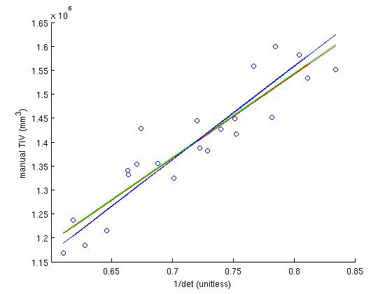
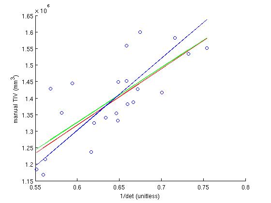
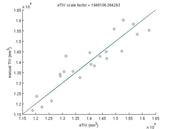
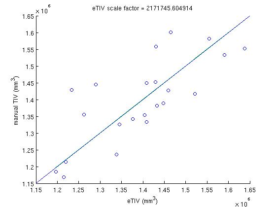
To determine the scaling factor, 22 subjects for which the TIV has been determined manually via their T2-weighted scans (which clearly show the skull), are used. These subjects are found in /space/freesurfer/subjects/atlases/SASHA. The scaling factor is determined analytically by first generating the determinant of the atlas transform for the 22 subjects, plotting this against each subjects manual TIV, fitting a line to this, and calculating the scale factor from the slope.

In that SASHA directory, in the the scripts directory, the script run_rb_xfm.csh will run the mri_label_volume binary and generate a matlab data file called det_eTIV_matdat.m which contains the determinant and eTIV data. Then, the matlab script plot_inv_det.m plots the inverse determinant against the manual TIV, finds the best fit to this plot, calculates the scale factor from that fit and then plots the eTIV against manual TIV, for each subject using that scaling factor. The file ICVnative_matdat.m contains the manual TIV data, copied from the ICVnative column in the file buckner_tiv.txt, which originates from the people performing the manual TIV measurements.

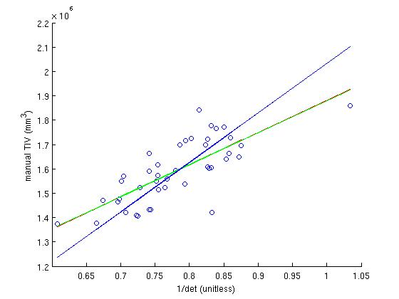
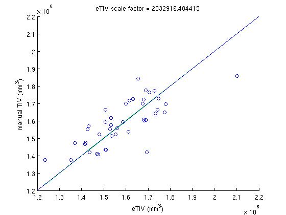
In the inverse determinant plots, the blue line is regression without y-intercept, and is used to determine the factor. For comparison, the green line is regression and the red line is robust regression with y intercept. The eTIV-manualTIV plots shows the comparison of the estimated and manual TIV's, were we hope to see the identity.

The eTIV was also assessed on two sets of longitudinal scans: a control and a patient undergoing atrophy. The scans were taken on three different platforms (Sonato and Avanto 1.5T and Trio 3T) and two different software versions (vb13 and vb15), over a period of six years. The max absolute relative error (in percent) and the average relative error were found to be:

• control:
  • all ten scans (Avanto and Trio): max 4.3%, mean 3.6%

  • Avanto vb13 & vb15 (seven scans): max 5.1%, mean 2.9%

  • Avanto vb15 (five scans): max 1% , mean 0.6%
• patient:
  • all 17 scans (Sonato, Avanto and Trio), from 2002 to 2008: max 3%, mean 1%
  • Sonata and Avanto vb13 and vb15 (16 scans), from 2002 to 2008: max 2.6%, mean 0.9%
  • Avanto vb13 and vb15 (13 scans), from 2004 to 2008: max 0.75%, mean 0.3%

This shows that even in the case of a patient known to be undergoing extensive atrophy, the eTIV variability is small and on par with the control.

ADNI T2 TIV

In the ADNI data set, an estimation of the TIV was conducted manually by Gloria Chiang of UCSF from T2 scans on 42 of the ADNI subjects. This alternate data allows a different estimation to be made of the scaling factor. The ADNI data is found at /autofs/eris/sabuncu/cluster/con/3/users/mert/ADNI, and a copy of the script run_rb_xfm.csh is found in the scripts dir. The raw data is in the file T2_TIV_data, which was transcribed to the file ICVnative_matdat.m to allow usage with the matlab script plot_inv_det.m. The output of running these scripts is shown in these plots (with SASHA results shown for comparison). The plots are described above in the Method section (note: the blue line is regression w/o y-intercept, and is used to determine the scale factor).

So the scaling factor differs, but the general trend of tiv vs inv_det is still there. Some measure of error needs to be made to compare the two datasets.